Changes in Buoyancy Detection

Joffrey JOUMAA

October 21, 2022

Here, the first thing to do is to retrieve the data processed at the end of vignette("data_exploration_2018").

# read the processed data
data_2018_filter <- readRDS("tmp/data_2018_filter.rds")

Daily median drift rate calculation

We then summarize the data by calculating the median of driftrate for each day.

# calulate the median of driftrate for each day
median_driftrate <- data_2018_filter[divetype == "2: drift",
  .(driftrate = quantile(driftrate, 0.5)),
  by = .(date = as.Date(date), .id)
]

# display 10 random rows
median_driftrate[sample(.N, 10), ] %>%
  sable(caption = "Median of daily drift rate by seals (10 random rows)")

Median of daily drift rate by seals (10 random rows)

date	.id	driftrate
2018-08-04	ind_2018074	-0.1900
2018-11-30	ind_2018080	-0.0950
2018-11-05	ind_2018072	0.1100
2018-05-28	ind_2018070	0.1675
2018-08-08	ind_2018072	-0.2300
2018-08-07	ind_2018070	-0.2150
2019-02-16	ind_2018074	-0.3000
2019-04-17	ind_2018074	-0.2825
2018-07-31	ind_2018080	-0.2150
2019-04-03	ind_2018072	-0.1425

# display the result
ggplot(
  median_driftrate,
  aes(x = date, y = driftrate, col = .id)
) +
  geom_point() +
  labs(y = "Daily drift rate (m/s)", x = "Date") +
  theme_jjo() +
  theme(legend.position = "top")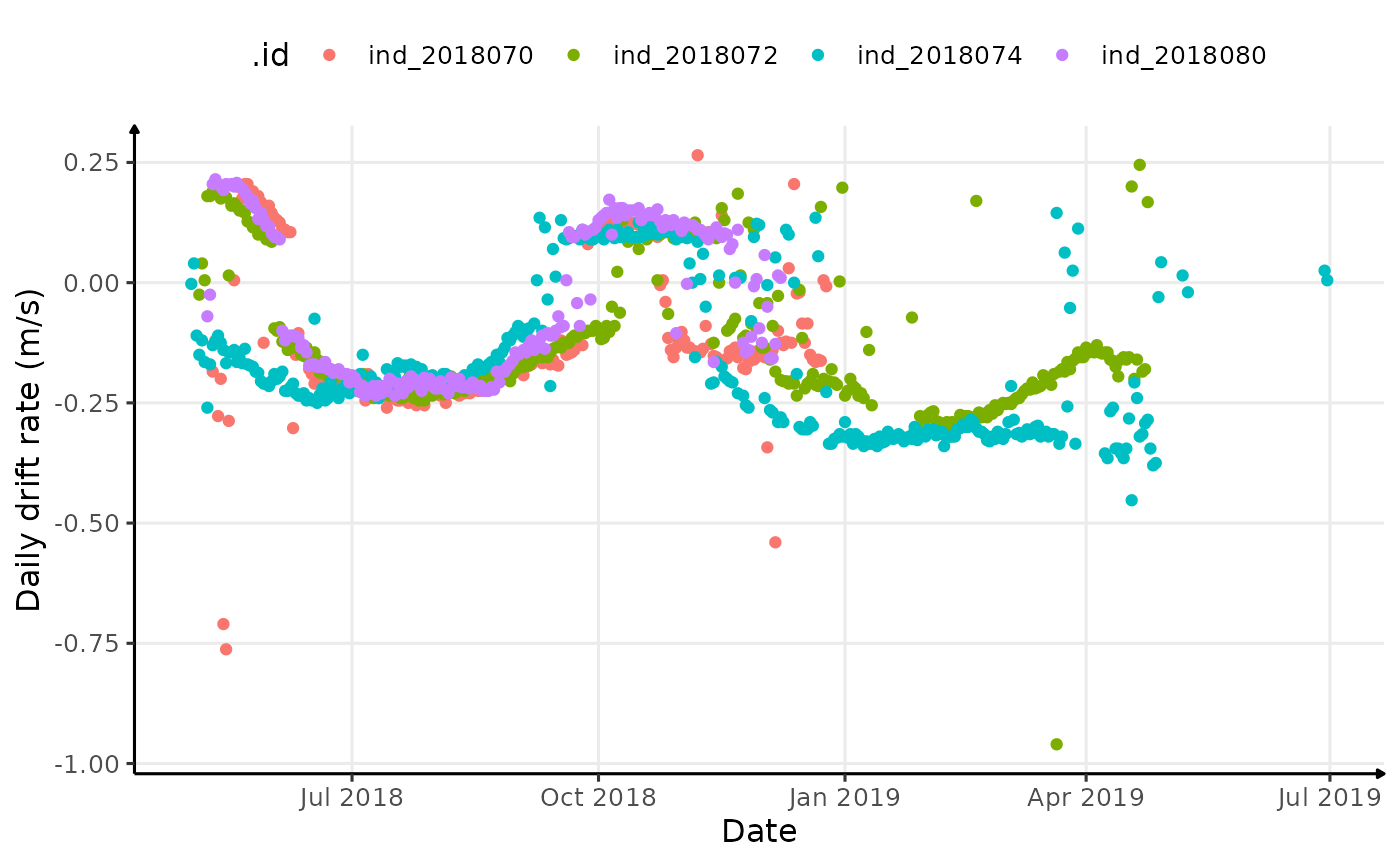

Evolution of daily median drift rate across time for each seals

Model daily median drift rate using a LOESS

For each seal, we model the daily median drift rate using a local polynomial regression.

The only parameter to estimate was the span, it was chosen graphically

# display the result
ggplot(
  median_driftrate,
  aes(x = date, y = driftrate, col = .id)
) +
  geom_point() +
  geom_smooth(span = 0.25, col = "black") +
  scale_x_date(date_labels = "%m/%Y") +
  labs(y = "Daily drift rate (m/s)", x = "Date") +
  theme_jjo() +
  theme(legend.position = "top") +
  facet_wrap(. ~ .id, scales = "free")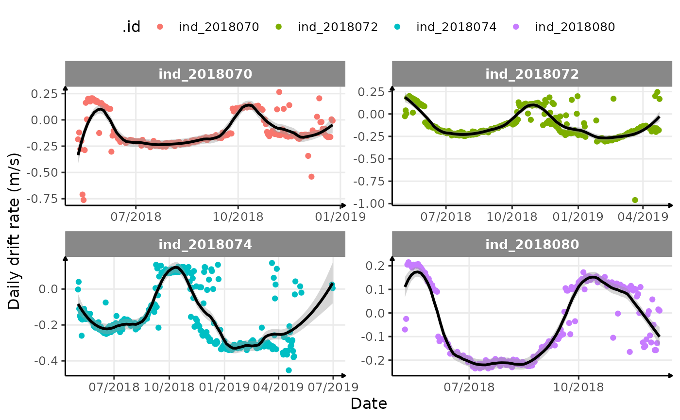

Evolution of daily median drift rate across time for each seals with a smooth

Detection of changes in buoyancy

We finally had to identify when the smooth function change sign.

# let's identity when the smooth changes sign
changes_driftrate <- median_driftrate %>%
  .[, .(
    y_smooth = predict(loess(driftrate ~ as.numeric(date), span = 0.25)),
    date
  ), by = .id] %>%
  .[c(FALSE, diff(sign(y_smooth)) != 0), ]

# display the result
ggplot(
  median_driftrate,
  aes(x = date, y = driftrate, col = .id)
) +
  geom_point() +
  geom_smooth(span = 0.25) +
  geom_vline(data = changes_driftrate, aes(xintercept = date)) +
  scale_x_date(date_labels = "%m/%Y") +
  labs(y = "Daily drift rate (m/s)", x = "Date") +
  theme_jjo() +
  theme(legend.position = "top") +
  facet_wrap(. ~ .id, scales = "free")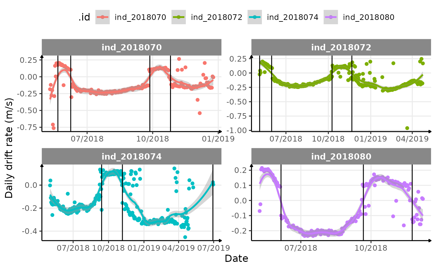

Evolution of daily median drift rate across time for each seals with a smooth and vertical lines to identify changes in buoyancy