Data Comparison - NES vs SES

Joffrey JOUMAA

October 21, 2022

Import Data

# load wealingNES package
library(weanlingNES)

# load dataset
data("data_nes")
data("data_ses")

# merge into one dataset
data_comp <- rbind(
  rbindlist(data_nes$year_2018),
  rbindlist(data_ses$year_2014),
  use.names = T,
  fill = T
)

# remove outlier (i.e. dive duration > 5000 s)
data_comp <- data_comp[dduration < 5000,]
data_comp[, diff_days := c(0,diff(day_departure)), by=.id]

# keep the first trip
data_comp_split = split(data_comp, by = c(".id"))
data_comp_split_list = lapply(data_comp_split, function(x){
  # calculate diff_days
  x[, diff_days := c(0,diff(day_departure)), by=.id]
  # find the rows after 100 day_departure where diff_days > 5
  date_cut = x[day_departure > 100 & diff_days > 1, min(date)]
  # return
  return(x[date < date_cut, ])
})
data_comp = rbindlist(data_comp_split_list)

# useful function to plot a dive profile based on animal ID and divenumber
plot_dive <- function(dataset){
  # retrieve ind
  ind = dataset[, unique(.id)]
  
  # retrieve the time of the beginning of the dive
  beg_date = dataset[, first(date)]
  
  # species
  species = dataset[, unique(sp)]
  
  # if its a ses
  if (species == "ses"){
    # retrieve file
    list_files = list.files("./inst/extdata/", 
                            pattern = "*iknos_raw_data.csv",
                            full.names = T)
    
    # find the one associated with ind
    file_ind = grep(ind, list_files, value=TRUE)
    
    # import file
    data = fread(file_ind, 
                 drop = "depth", 
                 col.names = c("depth","date"))
    
    # convert date
    data[, `:=` (date = matlab_to_posix(date, timez = "GMT"))]
  } else {
    # retrieve file
    list_files = list.files("./../Weanling Data/ucsc/Weanling Data GOOD/",
                            pattern = "*.csv",
                            recursive = T,
                            full.names = T)
    
    # find the one associated with ind
    files_ind = grep(paste0(substr(ind,5,11), "_nese0000annu_"), 
                     list_files, 
                     value=TRUE)
    
    # keep the shorter one
    file_ind = files_ind[which.min(unlist(lapply(files_ind,nchar)))]
    
    # import file
    data = fread(file_ind, 
                 drop = c("External Temperature", "Light Level"), 
                 col.names = c("date","time","depth"))
    
    # convert date
    data[, `:=` (date = as.POSIXct(paste(date, time), 
                                   format = "%d-%b-%Y %T",
                                   tz = "GMT"),
                 time = NULL)]
  }
  
  # plot
  p1 <- ggplot(data = data[date %between% c(beg_date, beg_date + (60 * 30)),], 
               aes(x = date, y = depth)) +
    scale_y_reverse() +
    geom_line() +
    labs(y = "Depth (m)",
         x = "Time",
         title = paste0(ind, " (", species, ") - ", beg_date))
  
  # return
  return(p1)
}

Plots

Proportion of Dives

# calculate the proportion of dive for each divetype, phase, sp, .id 
prop_dive_id_phase_divetype_sp <- data_comp[,table(divetype,sp,phase,.id)] %>% 
  # the calculate the proportion of dive in each divetype, per sp and phases
  prop.table(., c(".id")) %>% 
  # convert into a data.table
  as.data.table(.) 

# merge this table to add the number of dives, per divetype, phase, sp, .id
dataPlot <- merge(prop_dive_id_phase_divetype_sp,
                  data_comp[,.(nb_dives = uniqueN(divenumber)), 
                            by = .(divetype, sp , phase, .id)],
                  by = c("divetype","sp","phase",".id")) %>% 
  # mean + standard deviation
  .[, .(N = wtd.mean(N, nb_dives),
        N_sd = sqrt(wtd.var(N,nb_dives))), by = .(divetype,sp,phase)]

Result 1: Larger proportion of drift dives during the days compared to the night in nes, unlike ses Result 2: More transit in nes vs. more foraging in ses

# plot
ggplot(dataPlot, aes(x = divetype, y = N, fill = sp)) +
  geom_bar(stat = "identity", position = "dodge") +
  geom_errorbar(aes(ymin=N-N_sd, ymax=N+N_sd), width=.2,
                position=position_dodge(.9)) +
  scale_y_continuous(labels = label_percent()) +
  facet_grid(.~phase) +
  theme_jjo() +
  scale_fill_manual(values = c("#e08214", "#8073ac")) +
  labs(x = "Dive Types", y = "Average Proportion of Dives", fill = "Species") +
  theme(legend.position = "top",
        axis.line.x = element_line(arrow = NULL))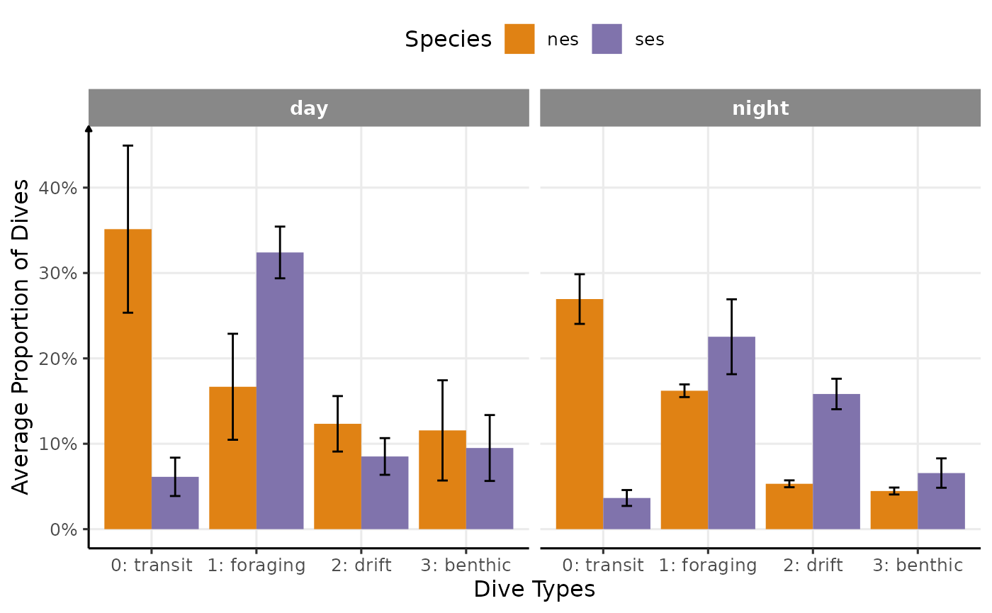

Proportion of dives by divetype, phases of the day and species (V1)

# plot
ggplot(dataPlot, aes(x = divetype, y = N, fill = phase)) +
  geom_bar(stat = "identity", position = "dodge", color="grey30") +
  geom_errorbar(aes(ymin=N-N_sd, ymax=N+N_sd), width=.2,
                position=position_dodge(.9)) +
  scale_y_continuous(labels = label_percent()) +
  facet_grid(.~sp) +
  theme_jjo() +
  # day first, and night
  scale_fill_manual(values = c("white", "grey")) +
  labs(x = "Dive Types", y = "Average Proportion of Dives") +
  theme(legend.position = "top",
        axis.line.x = element_line(arrow = NULL))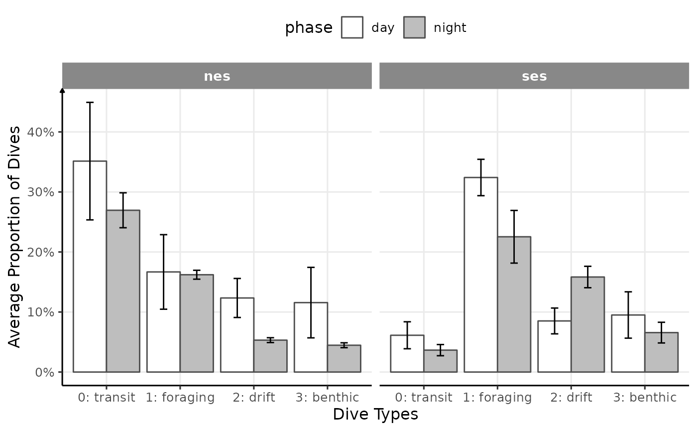

Proportion of dives by divetype, phases of the day and species (V2)

# plot
ggplot(copy(dataPlot)[sp=="nes",N:=-(1*N)], aes(x = divetype, y = N, fill = phase)) +
  geom_bar(stat = "identity", position = "dodge", color="grey30") +
  scale_y_continuous(labels = function(x) {percent(abs(x), 1)}) +
  geom_errorbar(aes(ymin=N-N_sd, ymax=N+N_sd), width=.2,
                position=position_dodge(.9)) +
  coord_flip() +
  facet_grid(.~sp, scales = "free_x") +
  theme_jjo() +
  # day first, and night
  scale_fill_manual(values = c("white", "grey")) +
  labs(x = "Dive Types", y = "Proportion of Dives") +
  theme(legend.position = "top",
        axis.line = element_line(arrow = NULL))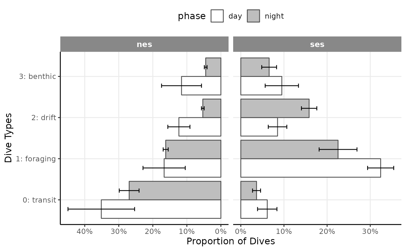

Proportion of dives by divetype, phases of the day and species (V3)

Max Depth

Let’s try to recreate the same plots Grecian, et al. (2022) did to compare the evolution of some behavioral parameters across time between nes and ses.

plot_comp(data_comp, "maxdepth", nb_days = 200, cols = "phase") +
  labs(
    x = "# days since departure",
    y = "Maximum Depth (m)",
    colour = "Species",
    fill = "Species"
  ) + 
  scale_y_reverse() +
  theme_jjo() +
  theme(legend.position = "top")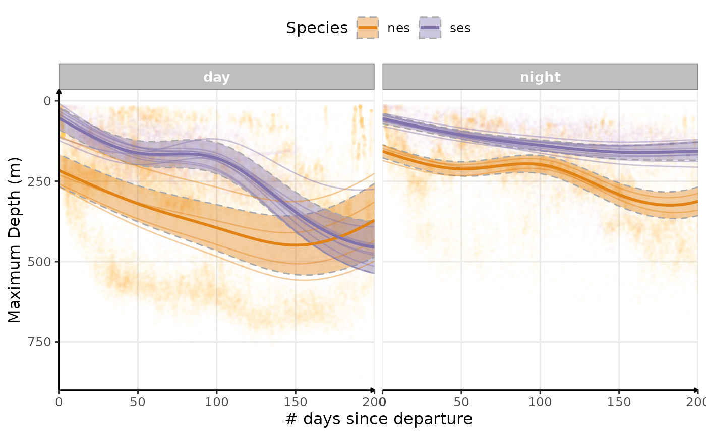

Estimated temporal changes in maximum depth (m) according to phases of the day

Since there is still this bimodality in the distribution of the maximumm depth during the day for nes, we splited by divetype.

• Points + Lines (phase ~ divetype)
• Only Lines (phase ~ divetype)
• Only Lines (sp ~ .)

plot_comp(data_comp, 
          "maxdepth", 
          nb_days = 200, 
          cols = "phase",
          rows = "divetype",
          scales = "free_y") +
  labs(
    x = "# days since departure",
    y = "Maximum Depth (m)",
    colour = "Species",
    fill = "Species"
  ) + 
  scale_y_reverse() +
  theme_jjo() +
  theme(legend.position = "top")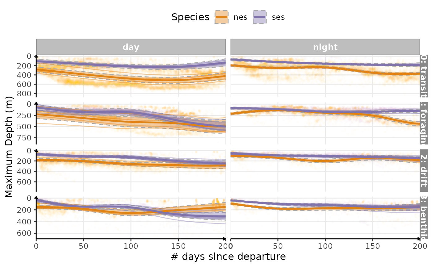

Estimated temporal changes in maximum depth (m) according to phases of the day and dive types (V1)

Still a bimodality in day for ses in transit dives…

plot_comp(data_comp, 
          "maxdepth", 
          nb_days = 200, 
          cols = "phase",
          rows = "divetype",
          scales = "free_y",
          point = FALSE) +
  labs(
    x = "# days since departure",
    y = "Maximum Depth (m)",
    colour = "Species",
    fill = "Species"
  ) + 
  scale_y_reverse() +
  theme_jjo() +
  theme(legend.position = "top")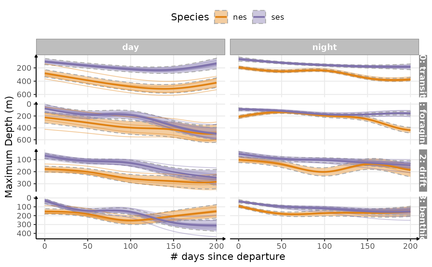

Estimated temporal changes in maximum depth (m) according to phases of the day and dive types (V2)

plot_comp(data_comp, 
          "maxdepth", 
          group_to_compare = "divetype",
          nb_days = 200, 
          cols = "sp",
          ribbon = T,
          point = F,
          scales = "free_y") +
  labs(
    x = "# days since departure",
    y = "Maximum Depth (m)",
    colour = "Species",
    fill = "Species"
  ) + 
  scale_y_reverse() +
  theme_jjo() +
  theme(legend.position = "top")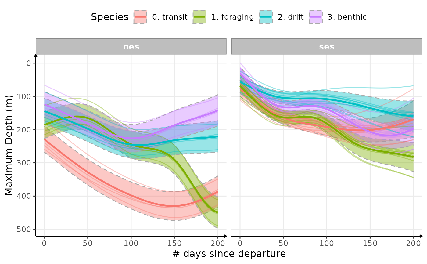

Estimated temporal changes in maximum depth (m) according to phases of the day and dive types (V3)

Dive Duration

plot_comp(data_comp, "dduration", nb_days = 200, cols = "phase") +
  labs(
    x = "# days since departure",
    y = "Dive Duration (s)",
    colour = "Species",
    fill = "Species"
  ) + 
  theme_jjo() +
  theme(legend.position = "top")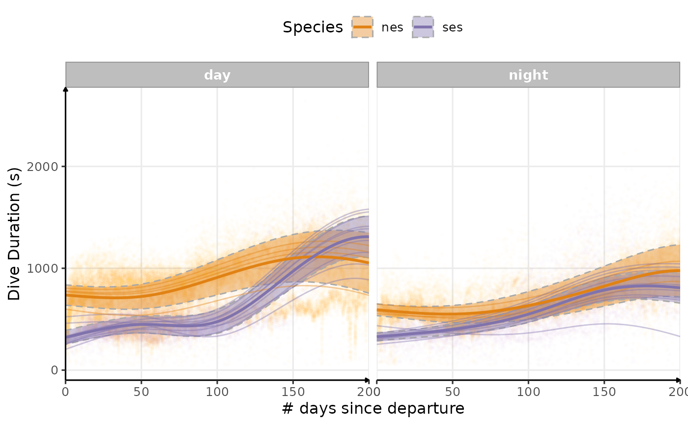

Estimated temporal changes in dive duration (s) according to phases of the day

plot_comp(data_comp, 
          "dduration", 
          nb_days = 200, 
          cols = "phase",
          rows = "divetype",
          scales = "free_y") +
  labs(
    x = "# days since departure",
    y = "Dive Duration (s)",
    colour = "Species",
    fill = "Species"
  ) + 
  theme_jjo() +
  theme(legend.position = "top")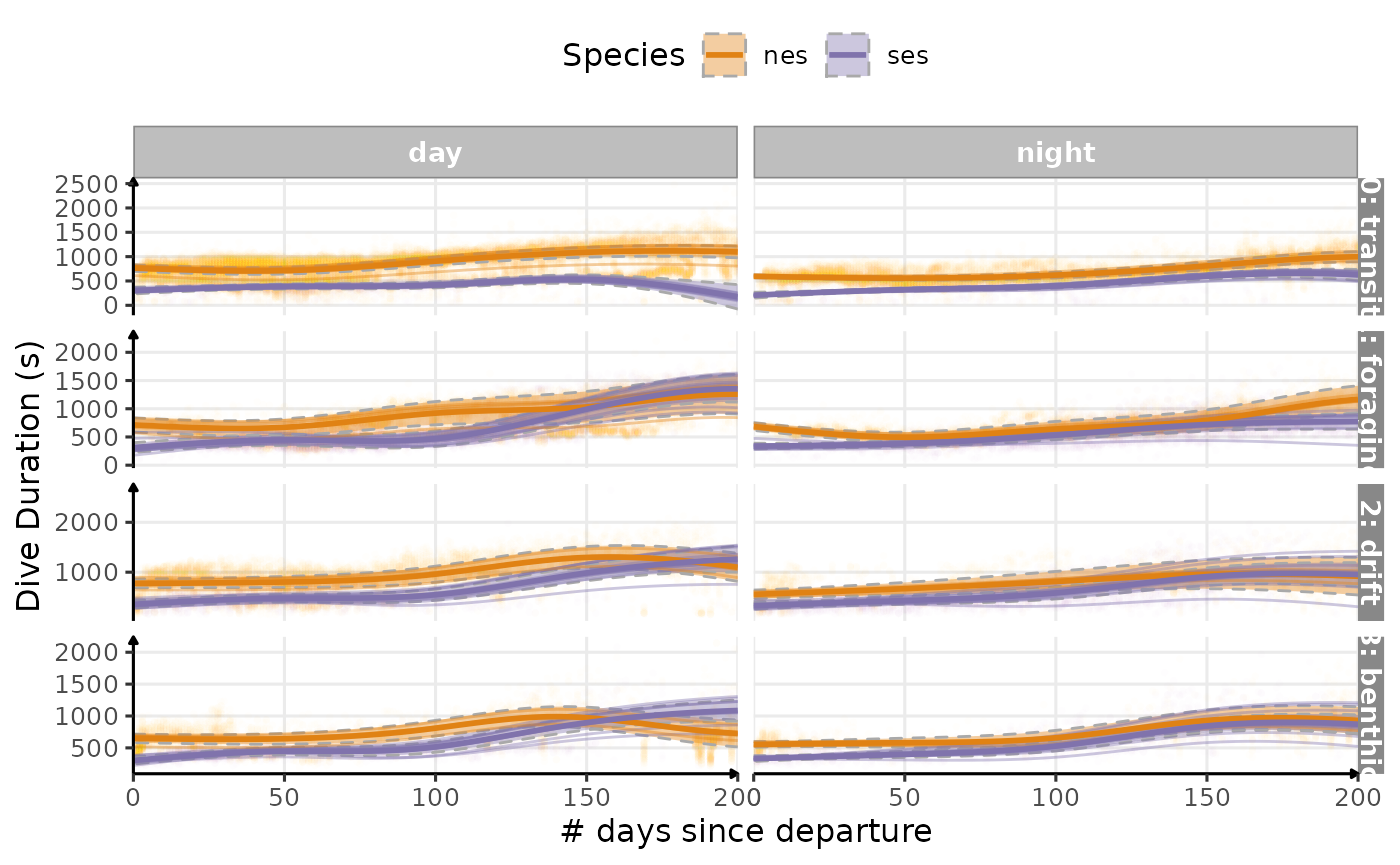

Estimated temporal changes in dive duration (s) according to phases of the day and dive types (V1)

plot_comp(data_comp, 
          "dduration", 
          group_to_compare = "divetype",
          nb_days = 200, 
          cols = "sp",
          ribbon = T,
          point = F,
          scales = "free_y",
          k = 7) +
  labs(
    x = "# days since departure",
    y = "Dive Duration (s)",
    colour = "Species",
    fill = "Species"
  ) + 
  theme_jjo() +
  theme(legend.position = "top")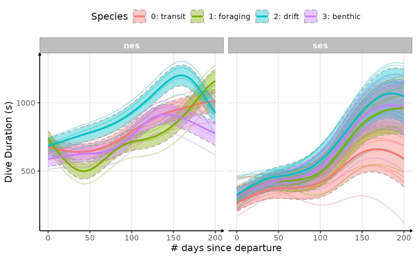

Estimated temporal changes in dive duration (s) according to phases of the day and dive types (V2)

“bADL”

# data nes
days_to_keep_nes = data_comp[sp=="nes",
                             .(nb_dives = .N),
                             by = .(.id, day_departure)] %>%
  .[nb_dives >= 50,]
# keep only those days
data_nes_complete_day = merge(data_comp[sp == "nes",],
                              days_to_keep_nes,
                              by = c(".id", "day_departure"))
# data ses
days_to_keep_ses = data_comp[sp=="ses",
                             .(nb_dives = .N),
                             by = .(.id, day_departure)] %>%
  .[nb_dives >= 8,]
# keep only those days
data_ses_complete_day = merge(data_comp[sp == "ses",],
                              days_to_keep_ses,
                              by = c(".id", "day_departure"))
# data plot
dataPlot = rbind(data_nes_complete_day[divetype=="1: foraging",
                                       .(badl = quantile(dduration, 0.95)),
                                       by = .(.id, day_departure, sp)],
                 data_ses_complete_day[divetype=="1: foraging",
                                       .(badl = quantile(dduration, 0.95)),
                                       by = .(.id, day_departure, sp)])

# comparative plot
plot_comp(dataPlot, "badl", nb_days = 200, alpha_point = .1) +
  labs(
    x = "# days since departure",
    y = "bADL (s)",
    col = "Species",
    fill = "Species"
  ) +
  theme_jjo()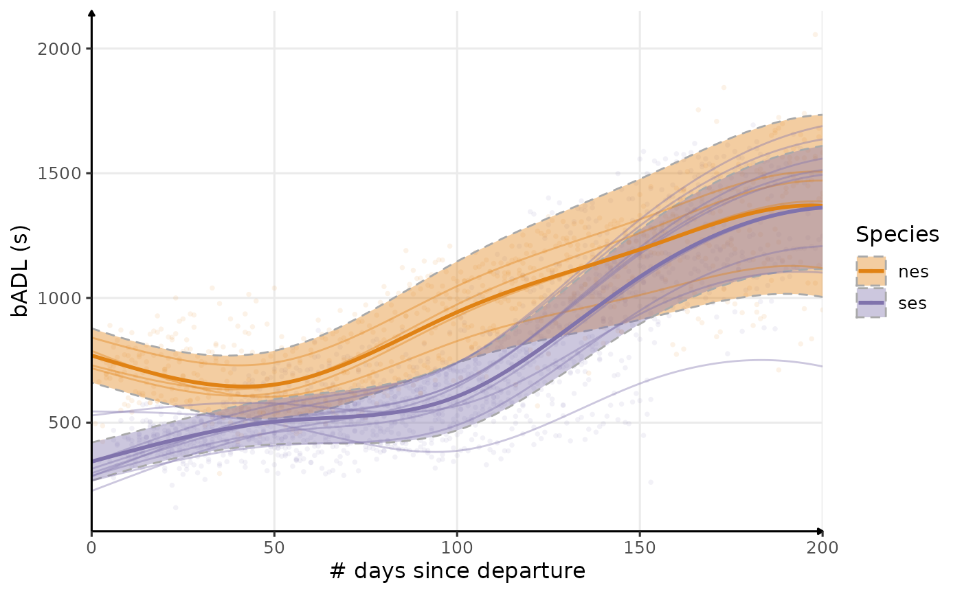

Estimated temporal changes in bADL (s)

Drift Rate

# calculate drift rate per day, id and sp
dataPlot = data_comp[divetype == "2: drift",
                     .(driftrate = quantile(driftrate, 0.5)),
                     by = .(day_departure, .id, sp)
]

# comparative plot
plot_comp(dataPlot, "driftrate", nb_days = 200, alpha_point = .1) +
  labs(
    x = "# days since departure",
    y = "Drift Rate (m/s)",
    title = "Day",
    col = "Species",
    fill = "Species"
  ) +
  theme_jjo() +
  theme(legend.position = "bottom")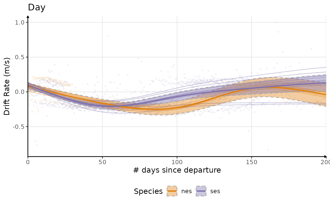

Estimated temporal changes in drift rate (m/s)

# comparative plot
plot_comp(dataPlot, "driftrate", nb_days = 200, alpha_point = .1, point = F) +
  labs(
    x = "# days since departure",
    y = "Drift Rate (m/s)",
    title = "Day",
    col = "Species",
    fill = "Species"
  ) +
  theme_jjo() +
  theme(legend.position = "bottom")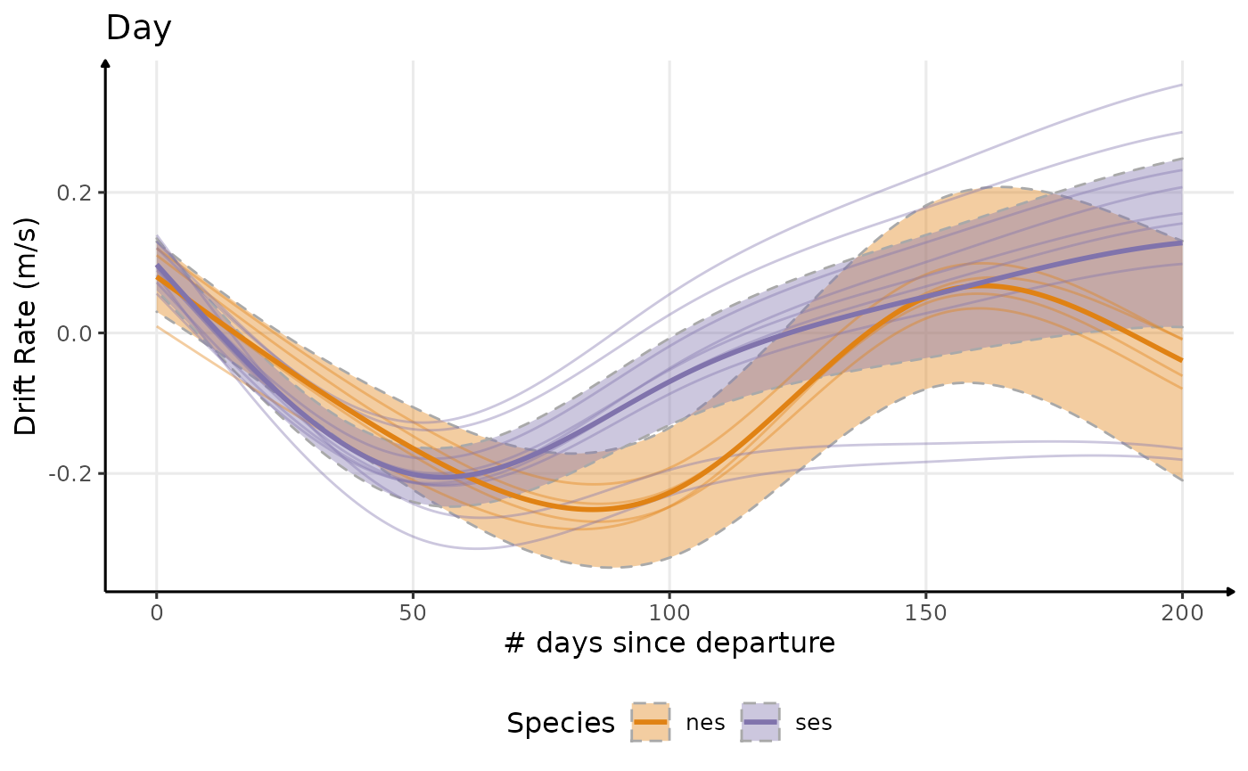

Maxdepth Bimodality Investigation

It’s weird that there is still a bimodality in the maxdepth’s distribution for northern elephant seal, even after splitting by phases of the day.

NES

To investigate why is that, let’s try several representation of this data for the individual 2018070 (nes).

# let's pick an individual
data_test <- data_comp[.id == "ind_2018070", ]

# first we average `lightatsurf` by individuals, day since departure and hour
dataPlot <- data_test[, .(lightatsurf = median(lightatsurf, na.rm = T),
                          phase = first(phase)),
                      by = .(.id,
                             day_departure,
                             date = as.Date(date),
                             hour)]

# then we choose the variable to represent
i <- "maxdepth"
ggplot(data = melt(data_test[, .(.id, date, get(i), phase)],
                   id.vars = c(".id",
                               "date",
                               "phase")),
       aes(x = as.Date(date),
           y = value,
           col = phase)) +
  geom_point(alpha = 1 / 10,
             size = .5) +
  facet_wrap(. ~ .id, scales = "free") +
  scale_x_date(date_labels = "%m/%Y") +
  labs(x = "Date", y = i) +
  scale_y_reverse() +
  theme_jjo() +
  theme(axis.text.x = element_text(angle = 45, hjust = 1),
        legend.position = "bottom") +
  guides(colour = guide_legend(override.aes = list(size = 7,
                                                   alpha = 1)))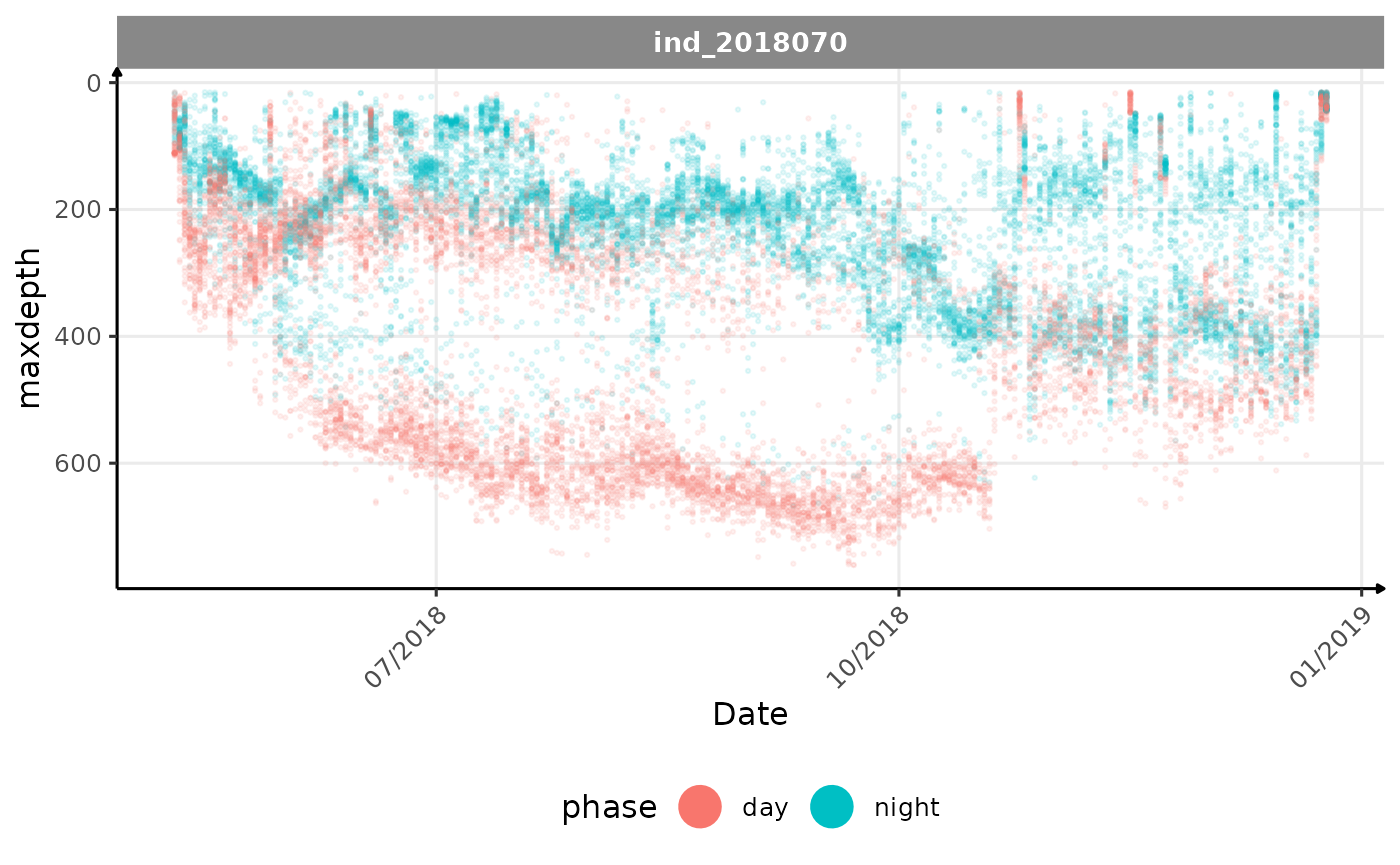

Evolution of the maximum depth reached across time for the individual 2018070

For this individual we can see that there are still a lot of shallow dives during the day. I first thought it was because this individual would probably have started reaching shallow water earlier in the day, at dusk, rather than waiting for complete darkness. To test this hypothesis, I tried to visualize the maxdepth over an entire day throughout the trip.

# this is art!
htmltools::tagList(
  plot_ly() %>%
    add_trace(
      data = data_test,
      x = ~hour,
      y = ~day_departure,
      z = ~maxdepth,
      marker = list(
        size = 1,
        opacity = 0.5
      ),
      mode = "markers",
      type = "scatter3d",
      text = ~divenumber,
      hovertemplate = paste(
        "Time: %{x:} h<br>",
        "Since departure: %{y:} days<br>",
        "Max Depth: %{z:} m<br>",
        "Dive Number: %{text:}"
      ),
      showlegend = FALSE
    ) %>% 
    add_trace(
      x = ~hour,
      y = ~day_departure,
      z = ~ (lightatsurf / 200) * 20,
      intensity = ~ lightatsurf / 200,
      data = dataPlot,
      type = "mesh3d",
      hovertemplate = paste(
        "Time: %{x:} h<br>",
        "Since departure: %{y:} days<br>",
        "Light Level: %{z:} ?"
      )
    ) %>%
    layout(
      scene = list(
        zaxis = list(title = "Maximum depth (m)",
                     autorange="reversed"),
        yaxis = list(title = "# days since departure"),
        xaxis = list(title = "Hour")
      ),
      legend = list(itemsizing = "constant")
    ) %>%
    hide_colorbar() %>% 
    config(modeBarButtons = list(list("toImage"),
                                 # list("editInChartStudio"),
                                 list("resetViews"),
                                 list("pan3d"), 
                                 list("orbitRotation"),
                                 list("tableRotation")))
)

We can see the bimodality of maxdepth within a day is not related to the time of the day, since swallow and deep dives might both occurred at the same time in the day. Let’s see what happen if we color dives with divetype.

# this is art!
htmltools::tagList(
  plot_ly() %>%
    add_trace(
      data = data_test,
      x = ~hour,
      y = ~day_departure,
      z = ~maxdepth,
      color = ~divetype,
      marker = list(
        size = 1,
        opacity = 0.5
      ),
      mode = "markers",
      type = "scatter3d",
      text = ~divenumber,
      hovertemplate = paste(
        "Time: %{x:} h<br>",
        "Since departure: %{y:} days<br>",
        "Max Depth: %{z:} m<br>",
        "Dive Number: %{text:}"
      )
    ) %>%
    add_trace(
      x = ~hour,
      y = ~day_departure,
      z = ~ (lightatsurf / 200) * 20,
      intensity = ~ lightatsurf / 200,
      data = dataPlot,
      type = "mesh3d",
      showlegend = FALSE,
      hovertemplate = paste(
        "Time: %{x:} h<br>",
        "Since departure: %{y:} days<br>",
        "Light Level: %{z:} ?"
      )
    ) %>%
    layout(
      scene = list(
        zaxis = list(title = "Maximum depth (m)",
                     autorange="reversed"),
        yaxis = list(title = "# days since departure"),
        xaxis = list(title = "Hour")
      ),
      legend = list(itemsizing = "constant")
    )  %>% 
    hide_colorbar() %>% 
    config(modeBarButtons = list(list("toImage"),
                                 # list("editInChartStudio"),
                                 list("resetViews"),
                                 list("pan3d"), 
                                 list("orbitRotation"),
                                 list("tableRotation")))
)

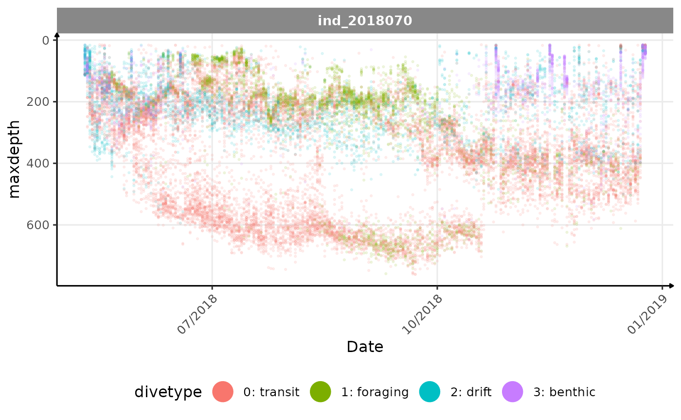
Well it seems that the bimodality observed in the distribution of maxdepth is mostly explained by divetype, with transit dives occurring at deeper dives that foraging and drift dives (at least for northern elephant seal). We can actually look at the same result with a simple 2D plot:

ggplot(
  data = melt(data_test[, .(.id, date, get(i), divetype)],
              id.vars = c(
                ".id",
                "date",
                "divetype"
              )
  ),
  aes(
    x = as.Date(date),
    y = value,
    col = divetype
  )
) +
  geom_point(
    alpha = 1 / 10,
    size = .5
  ) +
  facet_wrap(. ~ .id, scales = "free") +
  scale_x_date(date_labels = "%m/%Y") +
  labs(x = "Date", y = i) +
  theme_jjo() +
  scale_y_reverse() +
  theme(
    axis.text.x = element_text(angle = 45, hjust = 1),
    legend.position = "bottom"
  ) +
  guides(colour = guide_legend(override.aes = list(
    size = 7,
    alpha = 1
  )))

Kind of the same graph, but without looking at the hour of the day

And in bonus, we can add the bathymetry to the 3D plot.

htmltools::tagList(
  plot_ly() %>%
    add_trace(
      data = data_test,
      x = ~hour,
      y = ~day_departure,
      z = ~maxdepth,
      color = ~divetype,
      marker = list(
        size = 1,
        opacity = 0.5
      ),
      mode = "markers",
      type = "scatter3d",
      text = ~divenumber,
      hovertemplate = paste(
        "Time: %{x:} h<br>",
        "Since departure: %{y:} days<br>",
        "Max Depth: %{z:} m<br>",
        "Dive Number: %{text:}"
      ),
      legendgroup = 'group1',
      legendgrouptitle = list(text="Dive Types")
    ) %>%
    add_trace(
      x = ~hour,
      y = ~day_departure,
      z = ~ (lightatsurf / 200) * 20,
      intensity = ~lightatsurf,
      data = dataPlot,
      type = "mesh3d",
      legendgroup = "group2",
      name = "Light Level",
      showlegend = TRUE,
      hovertemplate = paste(
        "Time: %{x:} h<br>",
        "Since departure: %{y:} days<br>",
        "Light Level: %{z:} ?"
      )
    ) %>% 
    hide_colorbar() %>%
    add_trace(
      x = ~hour,
      y = ~day_departure,
      z = ~abs(bathy),
      color = "brown",
      name = "Bathymetry",
      data = data_test,
      type = "mesh3d",
      showlegend = TRUE,
      legendgroup = 'group2',
      legendgrouptitle = list(text="Other layers"),
      hovertemplate = paste(
        "Bathymetry: %{z:} m"
      )
    ) %>%
    layout(
      scene = list(
        zaxis = list(title = "Maximum depth (m)",
                     autorange="reversed"),
        yaxis = list(title = "# days since departure"),
        xaxis = list(title = "Hour")
      ),
      legend = list(itemsizing = "constant",
                    groupclick = "toggleitem")
    ) %>% 
    config(modeBarButtons = list(list("toImage"),
                                 # list("editInChartStudio"),
                                 list("resetViews"),
                                 list("pan3d"), 
                                 list("orbitRotation"),
                                 list("tableRotation")))
)

SES

Let’s do the same analysis on the individual 140059 (ses).

# let's pick an individual
data_test <- data_comp[.id == "ind_140059",]

# first we average `lightatsurf` by individuals, day since departure and hour
dataPlot <- data_test[, .(lightatsurf = median(lightatsurf, na.rm = T),
                          phase = first(phase)),
                      by = .(.id,
                             day_departure,
                             date = as.Date(date),
                             hour)]

# then we choose the variable to represent
i <- "maxdepth"
ggplot(data = melt(data_test[, .(.id, date, get(i), phase)],
                   id.vars = c(".id",
                               "date",
                               "phase")),
       aes(x = as.Date(date),
           y = value,
           col = phase)) +
  geom_point(alpha = 1 / 5,
             size = .5) +
  facet_wrap(. ~ .id, scales = "free") +
  scale_x_date(date_labels = "%m/%Y") +
  labs(x = "Date", y = i) +
  scale_y_reverse() +
  theme_jjo() +
  theme(axis.text.x = element_text(angle = 45, hjust = 1),
        legend.position = "bottom") +
  guides(colour = guide_legend(override.aes = list(size = 7,
                                                   alpha = 1)))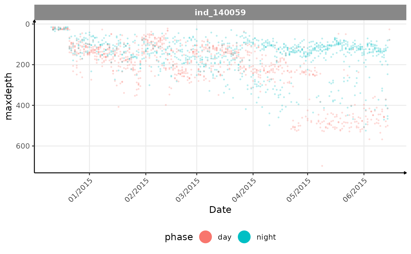

Evolution of the maximum depth reached across time for the individual 140059

ggplot(data = melt(data_test[, .(.id, date, get(i), divetype)],
                   id.vars = c(".id",
                               "date",
                               "divetype")),
       aes(x = as.Date(date),
           y = value,
           col = divetype)) +
  geom_point(alpha = 1 / 5,
             size = .5) +
  facet_wrap(. ~ .id, scales = "free") +
  scale_x_date(date_labels = "%m/%Y") +
  labs(x = "Date", y = i) +
  scale_y_reverse() +
  theme_jjo() +
  theme(axis.text.x = element_text(angle = 45, hjust = 1),
        legend.position = "bottom") +
  guides(colour = guide_legend(override.aes = list(size = 7,
                                                   alpha = 1)))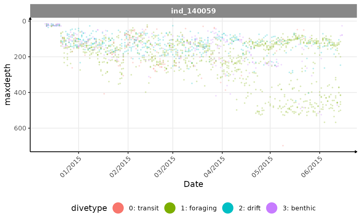

Evolution of the maximum depth reached across time for the individual 140059

For this individual we can see that until the half of its trip, there is no distinction between day and night in terms of maxdepth. But After, he starts to dive deeper during the day, and shallower during the night. Contrary to the previous nes individual, there seems to be a clear pattern. Let’s look at the graph in 3D:

htmltools::tagList(  
  plot_ly() %>%
    add_trace(
      data = data_test,
      x = ~hour,
      y = ~day_departure,
      z = ~maxdepth,
      color = ~divetype,
      marker = list(
        size = 1,
        opacity = 0.8
      ),
      mode = "markers",
      type = "scatter3d",
      text = ~divenumber,
      hovertemplate = paste(
        "Time: %{x:} h<br>",
        "Since departure: %{y:} days<br>",
        "Max Depth: %{z:} m<br>",
        "Dive Number: %{text:}"
      ),
      legendgroup = 'group1',
      legendgrouptitle = list(text="Dive Types")
    ) %>%
    add_trace(
      x = ~hour,
      y = ~day_departure,
      z = ~ (hour * 0.1) + 20,
      intensity = ~phase_bool,
      data = dataPlot[][, phase_bool := fifelse(phase == "night", 0, 1)][],
      type = "mesh3d",
      name = "Phases of the day",
      showlegend = TRUE,
      legendgroup = 'group2',
      legendgrouptitle = list(text="Other layers"),
      hovertemplate = paste(
        "Bathymetry: %{z:} m"
      )
    ) %>%
    add_trace(
      x = ~hour,
      y = ~day_departure,
      z = ~abs(bathy),
      color = "brown",
      name = "Bathymetry",
      data = data_test,
      type = "mesh3d",
      showlegend = TRUE,
      legendgroup = 'group2',
      legendgrouptitle = list(text="Other layers"),
      hovertemplate = paste(
        "Bathymetry: %{z:} m"
      )
    )  %>%
    hide_colorbar() %>% 
    layout(
      scene = list(
        zaxis = list(title = "Maximum depth (m)",
                     autorange = "reversed"),
        yaxis = list(title = "# days since departure"),
        xaxis = list(title = "Hour")
      ),
      legend = list(itemsizing = "constant",
                    groupclick = "toggleitem")
    )%>%
    config(modeBarButtons = list(list("toImage"),
                                 # list("editInChartStudio"),
                                 list("resetViews"),
                                 list("pan3d"),
                                 list("orbitRotation"),
                                 list("tableRotation")))
)