Figures
Joffrey JOUMAA
October 21, 2022
figures.Rmd1 Import Data
# load wealingNES package
library(weanlingNES)

# load dataset
data("data_nes")
data("data_ses")

# merge into one dataset
data_comp <- rbind(
  rbindlist(data_nes$year_2018),
  rbindlist(data_ses$year_2014),
  use.names = T,
  fill = T
)

# remove outlier (i.e. dive duration > 5000 s)
data_comp <- data_comp[dduration < 5000, ]
data_comp[, diff_days := c(0, diff(day_departure)), by = .id]

# keep the first trip
data_comp_split <- split(data_comp, by = c(".id"))
data_comp_split_list <- lapply(data_comp_split, function(x) {
  # find the rows after 100 day_departure where diff_days > 1
  second_trip <- x[day_departure > 100 & diff_days > 1, ]
  # if there is a second trip
  if (nrow(second_trip) != 0) {
    # get the first date of this second trip
    date_cut <- second_trip[, min(date)]
    # return only the first trip
    return(x[date < date_cut, ])
    # if no second trip
  } else {
    # return the full dataset
    return(x)
  }
})

# rebuilt the dataset
data_comp <- rbindlist(data_comp_split_list)

# rename sp for viz purposes
data_comp %>% .[, sp_rename := fifelse(
  sp == "nes",
  "Northern elephant seal",
  "Southern elephant seal"
)]
# rename divetype for viz purposes
data_comp[, divetype_rename := divetype %>%
            word(2) %>%
            str_to_title()]

# set up colours
# https://davidmathlogic.com/colorblind/#%23D81B60-%231E88E5-%23FFC107-%23004D40
# https://thenode.biologists.com/data-visualization-with-flying-colors/research/
# https://color.adobe.com/create/color-accessibility
# colours <- c("#e08214", "#8073ac")
colours <- c("#E1BE6A", "#009E73")
2 Figures
Figure 1
# datasets
data_fig_sum <- data_comp[!is.na(lat) & .id %in% c(
  "ind_2018070",
  "ind_140072"
), ] %>%
  .[.id == "ind_2018070", .id := "Northern elephant seal: ID 2018070"] %>%
  .[.id == "ind_140072", .id := "Southern elephant seal: ID 140072"] %>%
  .[, .id := ordered(.id, levels = c(
    "Northern elephant seal: ID 2018070",
    "Southern elephant seal: ID 140072"
  ))]

# maxdepth
data_fig_sum_maxdepth <- melt(
  data_fig_sum[, .(
    date,
    maxdepth,
    day_departure,
    .id
  )],
  id.vars = c("date", "day_departure", ".id"),
  measure.vars = c("maxdepth")
)

# duration
data_fig_sum_dduration <- melt(
  data_fig_sum[, .(
    date,
    dduration,
    day_departure,
    .id
  )],
  id.vars = c("date", "day_departure", ".id"),
  measure.vars = c("dduration")
)

# driftrate
data_fig_sum_driftrate <- melt(
  data_fig_sum[divetype == "2: drift", .(
    driftrate = median(driftrate, na.rm = T),
    day_departure = first(day_departure)
  ),
  by = .(date = as.Date(date), .id)
  ],
  id.vars = c("date", "day_departure", ".id"),
  measure.vars = c("driftrate")
)

# bADL
data_fig_sum_adl <- melt(
  data_fig_sum[divetype == "1: foraging",
               .(
                 adl = round(quantile(dduration, 0.95) /
                               60),
                 day_departure = first(day_departure)
               ),
               by = .(date = as.Date(date), .id)
  ],
  id.vars = c("date", "day_departure", ".id"),
  measure.vars = c("adl")
)

# configure theme (to get gradient https://encycolorpedia.com/)
nes_theme <- ttheme(
  colnames.style = colnames_style(
    color = "black",
    fill = colours[1],
    face = "bold"
  ),
  tbody.style = tbody_style(color = "black", fill = c("#e8c883", "#f3deb4"))
)
ses_theme <- ttheme(
  colnames.style = colnames_style(
    color = "black",
    fill = colours[2],
    face = "bold"
  ),
  tbody.style = tbody_style(color = "black", fill = c("#74bfa0", "#bbdfce"))
)
# read image
nes_image <- image_read("../man/figures/nes_crop.png")
ses_image <- image_read("../man/figures/ses_crop.png")

# map
trip <- basemap(
  shapefiles = "DecimalDegree",
  bathymetry = TRUE
) +
  geom_path(
    data = data_fig_sum,
    aes(x = lon, y = lat, group = .id),
    size = 2,
    colour = "white",
    show.legend = F
  ) +
  scale_fill_manual(
    name = "Bathymetry (m)",
    values = colorRampPalette(c(
      "#F7FBFF", "#DEEBF7", "#9ECAE1", "#4292C6", "#08306B"
    ))(10),
    labels =
      c(
        "0-50",
        "50-300",
        "300-500",
        "500-1000",
        "1000-1500",
        "1500-2000",
        "2000-4000",
        "4000-6000",
        "6000-10000",
        ">10000"
      )
  ) +
  geom_path(
    data = data_fig_sum,
    aes(x = lon, y = lat, col = .id),
    size = 1.5,
    show.legend = F
  ) +
  scale_color_manual(values = colours, guide = "none") +
  annotation_raster(nes_image, -175, -145, 20, 50) +
  annotation_raster(ses_image, 75, 105, -50, -20) +
  theme_void() +
  theme(legend.position = "top")

# maxdepth
fig_sum_maxdepth <-
  ggplot(data_fig_sum_maxdepth, aes(x = day_departure, y = value, col = .id)) +
  geom_point(
    show.legend = F,
    shape = 16,
    size = 1,
    alpha = 0.5
  ) +
  labs(y = "Maximum depth (m)") +
  scale_y_reverse() +
  scale_colour_manual(values = colours) +
  facet_grid2(. ~ .id,
              strip = strip_themed(background_x = elem_list_rect(fill = colours))
  ) +
  theme_jjo() +
  theme(
    axis.title.x = element_blank(),
    axis.text.x = element_blank(),
    axis.ticks.x = element_blank(),
    strip.background = element_blank(),
    strip.text.x = element_blank()
  )

# driftrate
fig_sum_dduration <-
  ggplot(
    data_fig_sum_dduration,
    aes(x = day_departure, y = value / 60, col = .id)
  ) +
  geom_point(
    show.legend = F,
    shape = 16,
    size = 1,
    alpha = 0.5
  ) +
  labs(y = "Dive duration (min)") +
  scale_colour_manual(values = colours) +
  facet_grid2(. ~ .id,
              strip = strip_themed(background_x = elem_list_rect(fill = colours))
  ) +
  theme_jjo() +
  theme(
    axis.title.x = element_blank(),
    axis.text.x = element_blank(),
    axis.ticks.x = element_blank(),
    strip.background = element_blank(),
    strip.text.x = element_blank()
  )

# driftrate
fig_sum_driftrate <-
  ggplot(
    data_fig_sum_driftrate,
    aes(x = day_departure, y = value, col = .id)
  ) +
  geom_point(show.legend = F) +
  geom_hline(
    yintercept = 0,
    linetype = "dashed",
    size = 1
  ) +
  labs(
    y = expression(paste("Daily median drift rate (m.", s^-1, ")")),
    x = "Number of days since departure"
  ) +
  scale_colour_manual(values = colours) +
  facet_grid2(. ~ .id,
              strip = strip_themed(background_x = elem_list_rect(fill = colours))
  ) +
  theme_jjo() +
  theme(
    strip.background = element_blank(),
    strip.text.x = element_blank()
  )
# summary table for nes
table_sum_nes <- data.table::transpose(data_fig_sum[sp == "nes", .(
  "# of days recorded" = prettyNum(
    uniqueN(as.Date(date)),
    big.mark = ",",
    scientific = FALSE
  ),
  "Recorder settings" = "All dives",
  "# of dives recorded" = prettyNum(.N, big.mark = ",", scientific = FALSE),
  "Median max depth" = paste(prettyNum(
    round(quantile(maxdepth, 0.5), 1),
    big.mark = ",",
    scientific = FALSE
  ), "m"),
  "Median dive duration" = paste(prettyNum(
    round(quantile(dduration, 0.5) / 60, 1),
    big.mark = ",",
    scientific = FALSE
  ), "min"),
  "Median bottom duration" = paste(prettyNum(
    round(quantile(botttime, 0.5) / 60, 1),
    big.mark = ",",
    scientific = FALSE
  ), "min")
), by = .("Seal ID" = .id)], keep.names = " ", make.names = 1)

# summary table for ses
table_sum_ses <- data.table::transpose(data_fig_sum[sp == "ses", .(
  "# of days recorded" = prettyNum(
    uniqueN(as.Date(date)),
    big.mark = ",",
    scientific = FALSE
  ),
  "Recorder settings" = "1 dive every ~2.25 hr",
  "# of dives recorded" = prettyNum(.N, big.mark = ",", scientific = FALSE),
  "Median max depth" = paste(prettyNum(
    round(quantile(maxdepth, 0.5), 1),
    big.mark = ",",
    scientific = FALSE
  ), "m"),
  "Median dive duration" = paste(prettyNum(
    round(quantile(dduration, 0.5) / 60, 1),
    big.mark = ",",
    scientific = FALSE
  ), "min"),
  "Median bottom duration" = paste(prettyNum(
    round(quantile(botttime, 0.5) / 60, 1),
    big.mark = ",",
    scientific = FALSE
  ), "min")
), by = .("Seal ID" = .id)], keep.names = " ", make.names = 1)

# format tables
table_sum_nes <- tableGrob(table_sum_nes,
                           rows = NULL,
                           cols = NULL,
                           theme = nes_theme
)
header_sum_nes <- tableGrob(mtcars[1, 1],
                            rows = NULL,
                            cols = c(data_fig_sum[sp == "nes", unique(.id)]),
                            theme = nes_theme
)
table_sum_nes <- gtable_combine(header_sum_nes[1, ], table_sum_nes, along = 2)
table_sum_nes$layout[1:2, c("r")] <- 2
table_sum_nes$widths <- unit(c(0.6, 0.4), "npc")

table_sum_ses <- tableGrob(table_sum_ses,
                           rows = NULL,
                           cols = NULL,
                           theme = ses_theme
)
header_sum_ses <- tableGrob(mtcars[1, 1],
                            rows = NULL,
                            cols = c(data_fig_sum[sp == "ses", unique(.id)]),
                            theme = ses_theme
)
table_sum_ses <- gtable_combine(header_sum_ses[1, ], table_sum_ses, along = 2)
table_sum_ses$layout[1:2, c("r")] <- 2
table_sum_ses$widths <- unit(c(0.6, 0.4), "npc")
# # final plot
# trip / (as_ggplot(table_sum_nes) + as_ggplot(table_sum_ses)) / fig_sum_maxdepth / fig_sum_dduration / fig_sum_driftrate +
#   # annotation A, B, C, ...
#   plot_annotation(tag_levels = list(c("(A)", "(B)", "", "(C)", "(D)", "(E)"))) +
#   # layout
#   plot_layout(heights = c(2, 1, 1, 1, 1)) &
#   # annotation in bold
#   theme(plot.tag = element_text(face = "bold"))
# # export (height 1375; width 875)
layout = "
AAAADDD
AAAADDD
AAAADDD
AAAAEEE
AAAAEEE
BBBBEEE
CCCCFFF
CCCCFFF
CCCCFFF
"

trip + guide_area() + (as_ggplot(table_sum_nes) + as_ggplot(table_sum_ses)) + fig_sum_maxdepth + fig_sum_dduration + fig_sum_driftrate +
  plot_annotation(tag_levels = list(c("(A)", "(B)", "", "(C)", "(D)", "(E)"))) +
  # layout
  plot_layout(design = layout, guides = 'collect') &
  # annotation in bold
  theme(plot.tag = element_text(face = "bold"))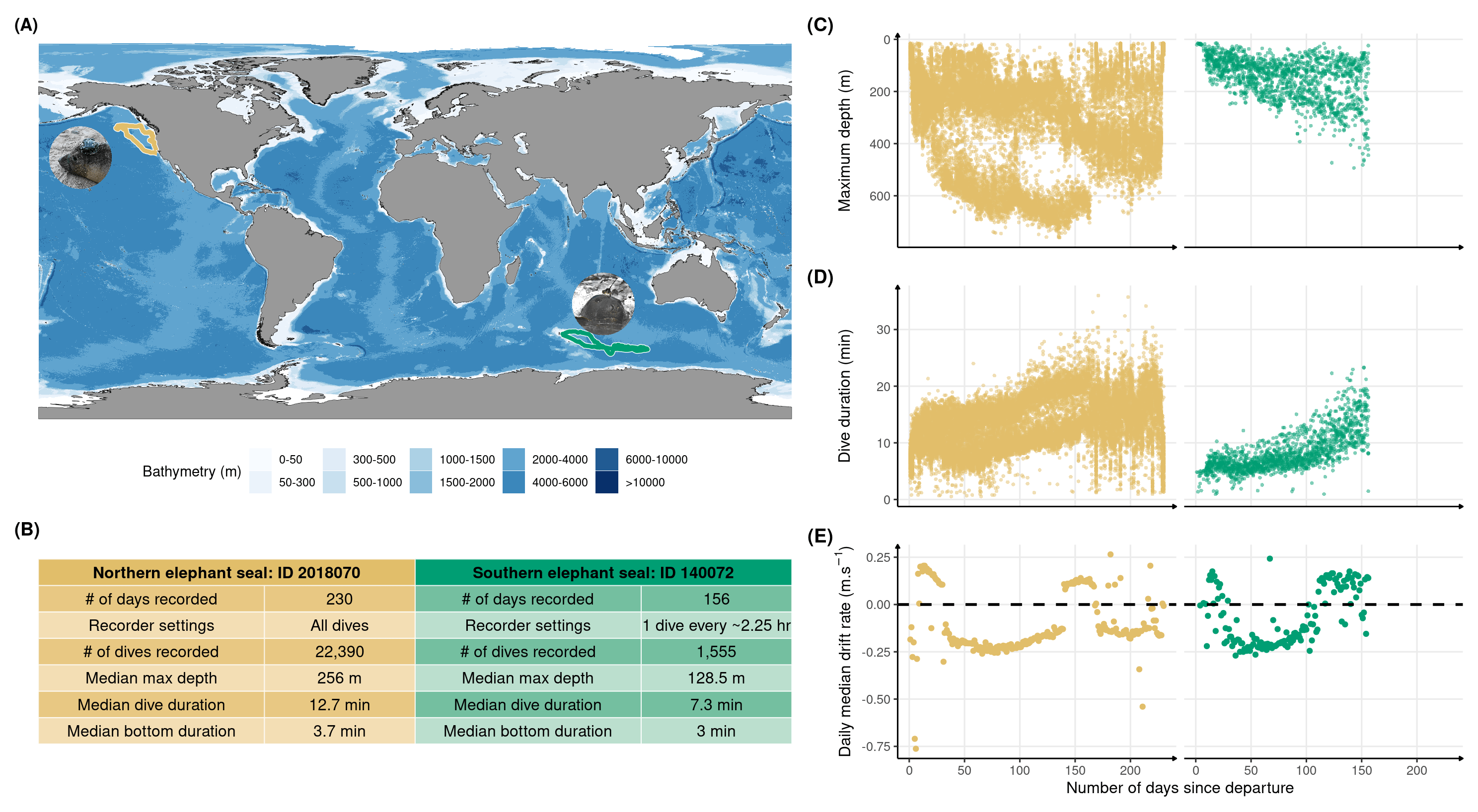
Figure 2.1: Illustrative data from one representative weanling northern elephant seal (2018070; gold) and one southern elephant seal (130072; green) for comparison. The panels show for each seal: (A) the migration routes during their first trip to sea from Año Nuevo, California, United States of America, and Kerguelen Island, France, respectively; (B) a summary of tag setup and dive characteristics; the development of (C) maximum diving depth, (D) dive duration, and (E) daily median drift rate. Data show clear improvement of diving physiology for both species, with northern elephant seals exhibiting accelerated development in both diving duration and depth.
# export (height 700; width 1450)Figure 2
# initial plots
fig_maxdepth_ini <- plot_comp(
  data_comp,
  "maxdepth",
  group_to_compare = "sp_rename",
  nb_days = 200,
  cols = "divetype_rename",
  ribbon = T,
  point = F,
  colours = colours,
  linetype_ribbon = 0,
  individual = FALSE,
  # method = "GCV.Cp",
  scales = "free_y"
)
fig_dduration_ini <- plot_comp(
  copy(data_comp)[, dduration_min := dduration / 60],
  "dduration_min",
  group_to_compare = "sp_rename",
  nb_days = 200,
  cols = "divetype_rename",
  ribbon = T,
  point = F,
  colours = colours,
  linetype_ribbon = 0,
  individual = FALSE,
  # method = "GCV.Cp",
  scales = "free_y"
)
# get limits
maxdepth_limits <- ggplot_build(fig_maxdepth_ini)$layout$panel_params[[1]]$y.range
dduration_limits <- ggplot_build(fig_dduration_ini)$layout$panel_params[[1]]$y.range

# update initial plots
fig_maxdepth <- fig_maxdepth_ini +
  labs(
    y = "Maximum depth (m)",
    colour = "Elephant seals",
    fill = "Elephant seals"
  ) +
  coord_cartesian(ylim = rev(maxdepth_limits)) +
  scale_colour_manual(
    values = colours,
    labels = data_comp[, sort(unique(sp_rename))] %>%
      word(1) %>%
      str_to_title()
  ) +
  scale_fill_manual(
    values = colours,
    labels = data_comp[, sort(unique(sp_rename))] %>%
      word(1) %>%
      str_to_title()
  ) +
  theme_jjo() +
  theme(
    legend.position = "top",
    axis.title.x = element_blank(),
    axis.text.x = element_blank(),
    axis.line.x = element_blank(),
    axis.ticks.x = element_blank(),
    strip.text = element_text(colour = 'grey20')
  )
fig_dduration <- fig_dduration_ini +
  labs(
    x = "Number of days since departure",
    y = "Dive duration (min)"
  ) +
  coord_cartesian(ylim = dduration_limits) +
  theme_jjo() +
  theme(
    legend.position = "none",
    strip.text.x = element_blank()
  )

# density plots
fig_dens_maxdepth <-
  ggplot(data_comp[day_departure <= 200, ], aes(y = maxdepth, fill = sp)) +
  geom_density(show.legend = F, col = "black", alpha = 0.4, size = 0.3) +
  coord_cartesian(ylim = rev(maxdepth_limits)) +
  scale_fill_manual(values = colours) +
  theme_void()
fig_dens_dduration <-
  ggplot(data_comp[day_departure <= 200, ], aes(y = dduration / 60, fill = sp)) +
  geom_density(show.legend = F, col = "black", alpha = 0.4, size = 0.3) +
  coord_cartesian(ylim = dduration_limits) +
  scale_fill_manual(values = colours) +
  theme_void()
((fig_maxdepth | fig_dens_maxdepth) + plot_layout(ncol = 2, widths = c(5, 1))) /
  ((fig_dduration | fig_dens_dduration) + plot_layout(ncol = 2, widths = c(5, 1)))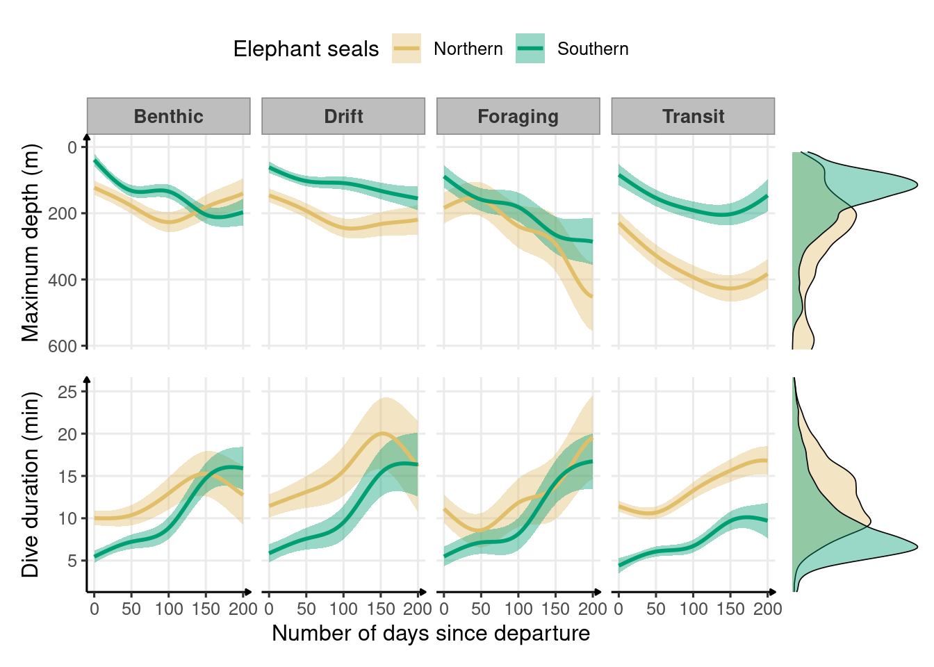
Figure 2.2: Development of depth and duration across dive types throughout the first trip to sea in northern (n=4) and southern elephant seals (n=9) estimated from generalized additive models. The solid lines represent the means, and the shaded areas represent the 95% confidence intervals. Marginal density plots represent the spread of data across all dive types for each species.
# Mann Whitney / Wilcoxon rank sum test on dive depth
tidy(wilcox.test(
  data_comp[day_departure <= 200 & sp == "nes", maxdepth],
  data_comp[day_departure <= 200 & sp == "ses", maxdepth]
)) %>%
  gt() %>%
tab_header(title = "Mann Whitney / Wilcoxon rank sum test on dive depth")| Mann Whitney / Wilcoxon rank sum test on dive depth | |||
| statistic | p.value | method | alternative |
|---|---|---|---|
| 902643075 | 0 | Wilcoxon rank sum test with continuity correction | two.sided |
# Mann Whitney / Wilcoxon rank sum test on dive duration
tidy(wilcox.test(
  data_comp[day_departure <= 200 & sp == "nes", dduration],
  data_comp[day_departure <= 200 & sp == "ses", dduration]
)) %>%
  gt() %>%
tab_header(title = "Mann Whitney / Wilcoxon rank sum test on dive duration")| Mann Whitney / Wilcoxon rank sum test on dive duration | |||
| statistic | p.value | method | alternative |
|---|---|---|---|
| 897660292 | 0 | Wilcoxon rank sum test with continuity correction | two.sided |
Figure 3
# (only for .id with location data, and so phase information)
prop_dive_id_phase_divetype_sp <- data_comp[
  !is.na(lat),
  table(divetype, sp, sp_rename, phase, .id)
] %>%
  # the calculate the proportion of dive in each divetype, per sp and phases
  prop.table(., c(".id")) %>%
  # convert into a data.table
  as.data.table(.)

# merge this table to add the number of dives, per divetype, phase, sp, .id
prop_dive_id_phase_divetype_sp <-
  merge(
    prop_dive_id_phase_divetype_sp,
    data_comp[!is.na(lat),
              .(nb_dives_divetype = uniqueN(divenumber)),
              by = .(sp, sp_rename, .id, divetype, phase)
    ] %>%
      .[, nb_dives := sum(nb_dives_divetype),
        by = .(.id)
      ] %>%
      .[],
    by = c("sp_rename", "sp", ".id", "divetype", "phase"),
    all.y = T
  )

# calculate the right proportions
dataPlot <- prop_dive_id_phase_divetype_sp %>%
  .[, .(
    N = wtd.mean(N, nb_dives),
    # its equivalent of using only the number of dives and not the percentage
    # N == N_v2
    N_v2 = sum(nb_dives_divetype) / sum(nb_dives),
    N_sd = sqrt(wtd.var(N, nb_dives))
  ),
  by = .(sp_rename, sp, divetype, phase)
  ]
# p_value calculation for nes
df_p_val_nes <- data_comp[sp == "nes" & !is.na(lat),
                          .(nb_divetype = .N),
                          by = .(divetype, phase)
] %>%
  .[, nb_dive := sum(nb_divetype)] %>%
  # perform by divetype
  rstatix::group_by(divetype) %>%
  # a prop.test test
  summarise(rstatix::prop_test(x = nb_divetype, n = nb_dive, correct = F)) %>%
  # then adjust the p_value for multiple test
  rstatix::adjust_pvalue(p.col = "p", method = "bonferroni") %>%
  # update p.adj
  rstatix::add_significance(p.col = "p.adj") %>%
  # sort
  arrange(divetype)

# dataset for nes
dataPlot_nes <- copy(dataPlot)[sp == "nes", N := -(1 * N)] %>%
  .[sp == "nes"]

# plot
fig_nes_prop <-
  ggplot(
    dataPlot_nes,
    aes(x = divetype, y = N, fill = phase)
  ) +
  geom_bar(
    stat = "identity",
    position = "dodge",
    color = "grey30"
  ) +
  scale_y_continuous(
    labels = function(x) {
      percent(abs(x), 1)
    }
  ) +
  geom_errorbar(aes(ymin = N - N_sd, ymax = N),
                width = .2,
                position = position_dodge(.9)
  ) +
  coord_flip(ylim = c(-c(round((dataPlot[, max(N + N_sd)] + 0.03) * 100) / 100, 0))) +
  facet_grid(. ~ sp_rename, scales = "free_x") +
  theme_jjo() +
  # day first, and night
  scale_fill_manual(
    values = c("white", "grey"),
    labels = c("Day-time", "Night-time")
  ) +
  # add stat
  geom_signif(
    y_position = dataPlot_nes[, .(position = min(N - N_sd)), divetype]$position +
      dataPlot_nes[, max(N + N_sd)] * 0.5,
    xmin = seq(0, dataPlot_nes[, uniqueN(divetype)] - 1) + 0.8,
    xmax = seq(1, dataPlot_nes[, uniqueN(divetype)]) + 0.2,
    # replace **** by *** (more standard)
    annotation = fifelse(
      df_p_val_nes$p.adj.signif == "****",
      "***",
      df_p_val_nes$p.adj.signif
    ),
    tip_length = 0,
    vjust = -0.6,
    angle = 90
  ) +
  labs(fill = "Time of day") +
  theme(
    legend.position = "top",
    axis.line.y = element_blank(),
    axis.title.y = element_blank(),
    axis.title.x = element_blank(),
    axis.text.y = element_blank(),
    axis.ticks.y = element_blank(),
    axis.line = element_line(arrow = arrow(
      length = unit(0.2, "lines"),
      type = "closed",
      ends = "first"
    )),
    strip.background = element_rect(fill = colours[1]),
    strip.text = element_text(colour = 'grey20')
  )

# p_value calculation for ses
df_p_val_ses <- data_comp[sp == "ses" & !is.na(lat),
                          .(nb_divetype = .N),
                          by = .(divetype, phase)
] %>%
  .[, nb_dive := sum(nb_divetype)] %>%
  # perform by divetype
  rstatix::group_by(divetype) %>%
  # a prop.test test
  summarise(rstatix::prop_test(x = nb_divetype, n = nb_dive, correct = F)) %>%
  # then adjust the p_value for multiple test
  rstatix::adjust_pvalue(p.col = "p", method = "bonferroni") %>%
  # update p.adj
  rstatix::add_significance(p.col = "p.adj") %>%
  # sort
  arrange(divetype)

# dataset for ses
dataPlot_ses <- copy(dataPlot)[sp == "ses", ] %>%
  .[sp == "ses"]

# plot
fig_ses_prop <-
  ggplot(dataPlot_ses, aes(x = divetype, y = N, fill = phase)) +
  geom_bar(
    stat = "identity",
    position = "dodge",
    color = "grey30"
  ) +
  scale_y_continuous(
    labels = function(x) {
      percent(abs(x), 1)
    }
  ) +
  geom_errorbar(aes(ymin = N, ymax = N + N_sd),
                width = .2,
                position = position_dodge(.9)
  ) +
  coord_flip(ylim = c(0, round((dataPlot[, max(N + N_sd)] + 0.03) * 100) / 100)) +
  facet_grid(. ~ sp_rename, scales = "free_x") +
  theme_jjo() +
  # day first, and night
  scale_fill_manual(
    values = c("white", "grey"),
    labels = c("Day-time", "Night-time")
  ) +
  # add stat
  geom_signif(
    y_position = dataPlot_ses[, .(position = max(N + N_sd)), divetype]$position +
      dataPlot_ses[, min(N + N_sd)] * 0.5,
    xmin = seq(0, dataPlot_ses[, uniqueN(divetype)] - 1) + 0.8,
    xmax = seq(1, dataPlot_ses[, uniqueN(divetype)]) + 0.2,
    # replace **** by *** (more standard)
    annotation = fifelse(
      df_p_val_ses$p.adj.signif == "****",
      "***",
      df_p_val_ses$p.adj.signif
    ),
    tip_length = 0
  ) +
  labs(fill = "Time of day") +
  theme(
    legend.position = "none",
    axis.line.y = element_blank(),
    axis.title.y = element_blank(),
    axis.title.x = element_blank(),
    axis.text.y = element_blank(),
    axis.ticks.y = element_blank(),
    axis.line.x = element_line(arrow = arrow(
      length = unit(0.2, "lines"), type = "closed"
    )),
    strip.background = element_rect(fill = colours[2]),
    strip.text = element_text(colour = 'grey20')
  )

df_text <- data.table(
  x = rep(0, data_comp[, uniqueN(divetype)]),
  label_to_order = data_comp[, sort(unique(divetype))],
  divetype = data_comp[, sort(unique(divetype))] %>%
    word(2) %>%
    str_to_title(),
  percentage = round(as.vector(prop.table(data_comp[
    !is.na(lat),
    table(divetype)
  ])) * 100, 1)
) %>%
  .[, label_to_display := paste0(divetype, "\n(", percentage, " %)")]
fig_text <-
  ggplot(df_text, aes(x = x, y = label_to_order, label = label_to_display)) +
  geom_text() +
  theme_void()

fig_label_1 <-
  ggplot(data.frame(l = "Percentage of dives", x = 1, y = 1)) +
  geom_text(aes(x, y, label = l)) +
  theme_void() +
  coord_cartesian(clip = "off")
((fig_nes_prop | fig_text | fig_ses_prop) +
   plot_layout(
     widths = c(4, 1, 4),
     guides = "collect"
   ) &
   theme(legend.position = "top")) / fig_label_1 +
  plot_layout(heights = c(6, 1))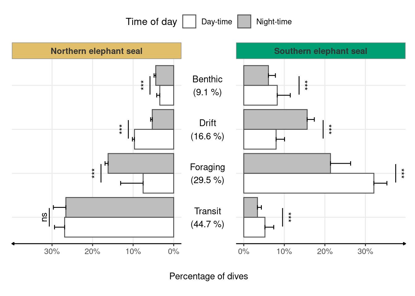
Figure 2.3: Frequency of dive types across time of day and species. Species-wide statistical test were based on averages of each individual’s dive type proportion weighted by the total number of dives. Percentages in the middle panel represent the frequency of each dive type across species and time of day. Asterisks indicate a significant difference (P-value<0.0001) between day-time and night-time dive frequencies within each species (two-sample z-test).
Figure 4
# calculate the median of driftrate for each day
median_driftrate <- data_comp[divetype == "2: drift",
                              .(driftrate = quantile(driftrate, 0.5)),
                              by = .(day_departure, .id, sp)
] %>%
  .[, sp := fifelse(sp == "nes", "Northern", "Southern")]

# initial plots
fig_driftrate_ini <- plot_comp(
  median_driftrate,
  "driftrate",
  group_to_compare = "sp",
  nb_days = 200,
  ribbon = T,
  linetype_ribbon = 0,
  point = F,
  colours = colours
)
# get limits
driftrate_limits <- ggplot_build(fig_driftrate_ini)$layout$panel_params[[1]]$y.range

# update initial plots
fig_driftrate <- fig_driftrate_ini +
  labs(
    y = expression(paste("Daily median drift rate (m.", s^-1, ")")),
    x = "Number of days since departure",
    colour = "Elephant seal",
    fill = "Elephant seal"
  ) +
  geom_hline(
    yintercept = 0,
    linetype = 2,
    size = 1,
    col = "black"
  ) +
  coord_cartesian(ylim = driftrate_limits) +
  theme_jjo() +
  theme(
    legend.position = "top"
  )

# density plots
fig_dens_driftrate <-
  ggplot(
    data_comp[divetype == "2: drift" & day_departure <= 200, ],
    aes(y = driftrate, fill = sp)
  ) +
  geom_density(show.legend = F, col = "black", alpha = 0.4, size = 0.3) +
  coord_cartesian(ylim = driftrate_limits) +
  scale_fill_manual(values = colours) +
  theme_void()
(fig_driftrate | fig_dens_driftrate) + plot_layout(widths = c(5, 1))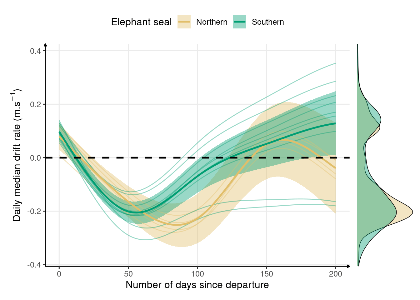
Figure 2.4: Changes in median drift rate across the first trip to sea in northern (n=4) and southern (n=9) elephant seals estimated from a generalized additive model. The bold solid lines represent the mean species-level responses while the thin lines represent individual-level responses. The shaded areas represent the 95% confidence interval, and the black dashed line indicates neutral buoyancy. Marginal density plots indicate the spread of data across the entire migration for each species.
Extra
data_comp[divetype == "2: drift",
          .(driftrate = median(driftrate, na.rm = T)),
          by = .(.id, day_departure, sp_rename)
] %>%
  merge(., data_comp[,
                     .(maxdepth = median(maxdepth, na.rm = T)),
                     by = .(.id, day_departure, sp_rename)
  ],
  by = c(".id", "day_departure", "sp_rename")
  ) %>%
  ggplot(aes(y = driftrate, x = maxdepth, col = word(sp_rename, 1))) +
  geom_point() +
  scale_color_manual(
    values = colours,
    name = "Elephant seals"
  ) +
  labs(
    x = "Daily median dive depth (m)",
    y = "Daily median drift rate (m/s)"
  ) +
  theme_jjo() +
  theme(legend.position = "top")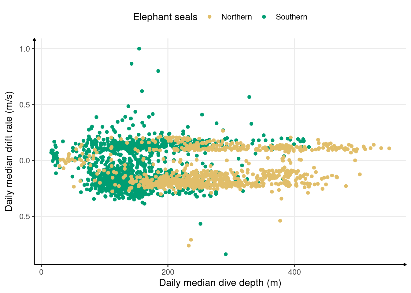
Figure 2.5: Daily median drift rate vs. daily median of maximum dive depth
data_comp[divetype == "2: drift",
          .(driftrate = median(driftrate, na.rm = T)),
          by = .(.id, day_departure, sp_rename)
] %>%
  merge(., data_comp[,
                     .(maxdepth = max(maxdepth, na.rm = T)),
                     by = .(.id, day_departure, sp_rename)
  ],
  by = c(".id", "day_departure", "sp_rename")
  ) %>%
  ggplot(aes(y = driftrate, x = maxdepth, col = word(sp_rename, 1))) +
  geom_point() +
  scale_color_manual(
    values = colours,
    name = "Elephant seals"
  ) +
  labs(
    x = "Daily maximum dive depth (m)",
    y = "Daily median drift rate (m/s)"
  ) +
  theme_jjo() +
  theme(legend.position = "top")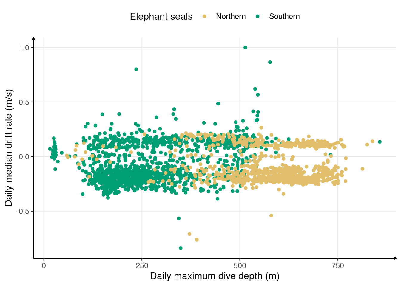
Figure 2.6: Daily median drift rate vs. daily maximum of maximum dive depth
From these two graphs, I don’t think it can be said that somehow body condition constrains dive depth, since deep dives occur at positive and negative buoyancies.
3 Tables
Table 1
I thought about doing a table that provides summary information and gives a rapid overview of the dataset.
# based on
# https://themockup.blog/posts/2020-10-31-embedding-custom-features-in-gt-tables/
gt_ggplot_driftrate <- function(table_data, plot_col, data_col, plot_fun, ...) {
  # save the data extract ahead of time
  # to be used in our anonymous function below
  data_in <- purrr::pluck(table_data, "_data", data_col)

  # retrieve min max
  range_x <- rbindlist(data_in)[, range(day_departure)]
  range_y <- c(-0.35, 0.15)

  # draw plot
  text_transform(
    table_data,
    # note the use of {{}} here - this is tidy eval
    # that allows you to indicate specific columns
    locations = cells_body(columns = c({{ plot_col }})),
    fn = function(x) {
      # build the plot
      plot <- lapply(data_in, function(x) {
        # build the plot
        ggplot(x) +
          # for color https://davidmathlogic.com/colorblind/#%23D81B60-%231E88E5-%23FFC107-%23004D40
          geom_area(aes(x = day_departure, y = ifelse(driftrate < 0,
                                                      driftrate, 0)),
                    fill = "#5D3A9B", alpha = 0.5
          ) +
          # for color https://davidmathlogic.com/colorblind/#%23D81B60-%231E88E5-%23FFC107-%23004D40
          geom_area(aes(x = day_departure, y = ifelse(driftrate > 0,
                                                      driftrate, 0)),
                    fill = "#E66100", alpha = 0.5
          ) +
          geom_segment(aes(x = 0,
                           y = 0,
                           xend = max(day_departure) + 10 ,
                           yend = 0),
                       size = 7,
                       colour = "grey30",
                       arrow = arrow(type = "closed",
                                     length = unit(0.2, units = "npc"))) +
          coord_cartesian(xlim = range_x, ylim = range_y) +
          theme_void() +
          theme(
            panel.grid = element_blank(),
            panel.border = element_blank(),
          )
      })

      # draw for every row
      lapply(plot, ggplot_image, aspect_ratio = 5, height = 25)
    }
  )
}
gt_ggplot_sparkline <- function(table_data, plot_col, data_col, plot_fun, ...) {
  # save the data extract ahead of time
  # to be used in our anonymous function below
  data_in <- purrr::pluck(table_data, "_data", data_col)

  # colnames
  col_names <- colnames(rbindlist(data_in))

  # interest variable
  var_interest <- setdiff(col_names, "day_departure")

  # retrieve min max
  range_x <- rbindlist(data_in)[, range(day_departure)]
  range_y <- rbindlist(data_in)[, range(get(var_interest))]

  # draw plot
  text_transform(
    table_data,
    # note the use of {{}} here - this is tidy eval
    # that allows you to indicate specific columns
    locations = cells_body(columns = c({{ plot_col }})),
    fn = function(x) {
      # build the plot
      plot <- lapply(data_in, function(x) {
        # build the plot
        ggplot(x, aes(x = day_departure, y = get(var_interest))) +
          geom_path(size = 6, color = "grey60") +
          geom_smooth(size = 10,
                      linetype = "dashed",
                      colour = "black",
                      method = "lm",
                      se = FALSE,
                      na.rm = TRUE) +
          coord_cartesian(xlim = range_x, ylim = range_y) +
          theme_void() +
          theme(
            panel.grid = element_blank(),
            panel.border = element_blank()
          )
      })

      # draw for every row
      lapply(plot, ggplot_image, aspect_ratio = 4, height = 26)
    }
  )
}
# summary_table_es <-
data_comp[, travel_distance := distGeo(
  matrix(c(lon, lat), ncol = 2),
  matrix(c(shift(lon), shift(lat)), ncol = 2)
),
by = .id
] %>%
  as_tibble() %>%
  mutate(id_rename = word(.id, 2, sep = "_")) %>%
  group_by(sp_rename, id_rename) %>%
  summarise(
    N = prettyNum(n(),
                  big.mark = ",",
                  scientific = FALSE
    ),
    nb_days = round(as.numeric(difftime(
      last(date), first(date),
      units = "days"
    )), 1),
    travel_distance = prettyNum(
      sum(travel_distance, na.rm = T) / 1000,
      digits = 1,
      big.mark = ",",
      scientific = FALSE
    ),
    Maxdepth_mean = round(mean(maxdepth),1),
    Maxdepth_plus_minus = "±",
    Maxdepth_sd = round(sd(maxdepth),1),
    Dduration_mean = round(mean(dduration)/60,1),
    Dduration_plus_minus = "±",
    Dduration_sd = round(sd(maxdepth)/60,1),
    .groups = "drop"
  ) %>%
  # replace travel_distance = 0 by NA
  mutate(travel_distance = na_if(travel_distance, 0)) %>%
  # add driftrate from drift dives
  left_join(
    .,
    data_comp %>%
      as_tibble() %>%
      mutate(id_rename = word(.id, 2, sep = "_")) %>%
      group_by(sp_rename, id_rename, day_departure) %>%
      filter(divetype == "2: drift") %>%
      summarise(
        driftrate = as.numeric(quantile(
          driftrate, 0.5,
          na.rm = T
        )),
        .groups = "drop"
      ) %>%
      group_by(sp_rename, id_rename) %>%
      summarise(
        sparkline_driftrate = list(
          data.frame(
            driftrate = driftrate,
            day_departure = day_departure
          )
        ),
        .groups = "drop"
      ),
    by = c("sp_rename", "id_rename")
  ) %>%
  # add quantile 95 of dduration and max_depth
  left_join(
    .,
    data_comp %>%
      as_tibble() %>%
      mutate(id_rename = word(.id, 2, sep = "_")) %>%
      group_by(sp_rename, id_rename, day_departure) %>%
      summarise(
        maxdepth = as.numeric(quantile(maxdepth, 0.95, na.rm = T)),
        dduration = as.numeric(quantile(dduration, 0.95, na.rm = T)),
        .groups = "drop"
      ) %>%
      group_by(sp_rename, id_rename) %>%
      summarise(
        sparkline_qt_dduration = list(
          data.frame(
            dduration = dduration,
            day_departure = day_departure
          )),
        sparkline_qt_maxdepth = list(
          data.frame(
            maxdepth = -maxdepth,
            day_departure = day_departure
          )),
        .groups = "drop"
      ),
    by = c("sp_rename", "id_rename")
  ) %>%
  # add percentage
  left_join(
    .,
    data_comp %>%
      as_tibble() %>%
      mutate(id_rename = word(.id, 2, sep = "_")) %>%
      group_by(sp_rename, id_rename, divetype) %>%
      summarise(
        n = n(),
        .groups = "drop"
      ) %>%
      group_by(sp_rename, id_rename) %>%
      summarise(
        divetype_perc = round(n * 100 / sum(n)),
        divetype,
        .groups = "drop"
      ) %>%
      arrange(divetype) %>%
      group_by(sp_rename, id_rename) %>%
      summarise(divetype_perc = list(divetype_perc), .groups = "drop"),
    by = c("sp_rename", "id_rename")
  ) %>%
  # add wean mass based on Weanling Dive Metada.xlsx
  left_join(
    .,
    data.table(
      id_rename = c(
        "2018070",
        "2018072",
        "2018074",
        "2018080",
        "140059",
        "140060",
        "140062",
        "140063",
        "140068",
        "140069",
        "140072",
        "140073",
        "140075"
      ),
      sp_rename = c(
        rep("Northern elephant seal", 4),
        rep("Southern elephant seal", 9)
      ),
      weanmass = c(132, 138, 119, 142, 118, 112, 85, NA, 125, NA, NA, 102, NA)
    ),
    by = c("sp_rename", "id_rename")
  ) %>%
  # reorder column
  relocate(nb_days, N, travel_distance, weanmass, divetype_perc,
           .after = id_rename) %>%
  # setup group row
  gt(groupname_col = "sp_rename") %>%
  # spanner (several columns into one column)
  tab_spanner(
    label = "Maximum depth (m)",
    columns = c(
      Maxdepth_mean,
      Maxdepth_plus_minus,
      Maxdepth_sd,
      sparkline_qt_maxdepth
    )
  ) %>%
  tab_spanner(
    label = "Dive duration (min)",
    columns = c(
      Dduration_mean,
      Dduration_plus_minus,
      Dduration_sd,
      sparkline_qt_dduration
    )
  ) %>%
  tab_spanner(
    label = md("Daily median drift rate"),
    columns = c(sparkline_driftrate)
  ) %>%
  tab_spanner(
    label = md("Travel distance"),
    columns = c(travel_distance)
  ) %>%
  tab_spanner(
    label = md("Weaning mass"),
    columns = c(weanmass)
  ) %>%
  tab_spanner(
    label = md("Dive type proportions"),
    columns = c(divetype_perc)
  ) %>%
  # plot
  gt_ggplot_sparkline(sparkline_qt_maxdepth, "sparkline_qt_maxdepth") %>%
  gt_ggplot_sparkline(sparkline_qt_dduration, "sparkline_qt_dduration") %>%
  gt_ggplot_driftrate(sparkline_driftrate, "sparkline_driftrate") %>%
  gt_plt_bar_stack_extra(
    divetype_perc,
    width = 65,
    labels = c("Transit", "Foraging", "Drift", "Benthic"),
    palette = c("#000000", "#444444", "#888888", "#CCCCCC")
  ) %>%
  # alignement
  cols_align(
    columns = c(N, Maxdepth_sd, Dduration_sd),
    align = "left"
  ) %>%
  cols_align(
    columns = c(N, Maxdepth_mean, Dduration_mean),
    align = "right"
  ) %>%
  cols_align(
    columns = c(travel_distance, weanmass, Maxdepth_plus_minus, Dduration_plus_minus),
    align = "center"
  ) %>%
  # format
  fmt_number(
    columns = Maxdepth_mean,
    decimal = 1
  ) %>%
    fmt_number(
    columns = ends_with("_sd"),
    decimal = 1
  ) %>%
  # rename columns
  cols_label(
    N = "# dives",
    id_rename = md("ID"),
    nb_days = "# days",
    travel_distance = "(km)",
    weanmass = "(kg)",
    Maxdepth_mean = md("Mean"),
    Maxdepth_plus_minus = md("±"),
    Maxdepth_sd = md("SD"),
    sparkline_qt_maxdepth = md("Trend"),
    Dduration_mean = md("Mean"),
    Dduration_plus_minus = md("±"),
    Dduration_sd = md("SD"),
    sparkline_driftrate = md("(m.s<sup>-1</sup>)"),
    sparkline_qt_dduration = md("Trend")
  ) %>%
  # add color square
  text_transform(
    locations = cells_row_groups(),
    fn = function(x) {
      # identify sp
      sp <- unique(x)
      # set colour
      colour <-
        if_else(grepl("Northern", sp), colours[1], colours[2])
      # html to add the color box
      purrr::map(x, ~ html(
        glue(
          "<div><span style='height: 15px;width: 15px;background-color: {colour};display: inline-block;border-radius:5px;float:left;top:13%;left:5%;'</span> <span style='display: inline-block;float:left;line-height:20px;padding: 0px 25px;white-space:nowrap;'>{sp}</span></div>"
        )
      ))
    }
  ) %>%
  # color cols
  gt_highlight_cols(
    columns = c(
      Maxdepth_mean,
      Maxdepth_plus_minus,
      Maxdepth_sd,
      sparkline_qt_maxdepth,
      sparkline_driftrate,
      weanmass,
      N
    ),
    fill = "lightgrey",
    alpha = 0.5
  ) %>%
  # footnote
  tab_footnote(
    footnote = "Recorded",
    locations = cells_column_labels(columns = c(N, nb_days))
  ) %>%
  # color rows
  opt_row_striping() %>%
  # set horizontal padding for plus minus
  tab_style(style = "padding-left:0px;padding-right:0px;",
            locations = cells_column_labels(columns = ends_with("plus_minus"))) %>%
      tab_style(style = "padding-left:0px;padding-right:0px;",
            locations = cells_body(columns = ends_with("plus_minus"))) %>%
  # set horizontal padding for plus minus
  tab_style(style = "padding-top:0px;padding-bottom:0px",
            locations = cells_body(columns = starts_with("sparkline"))) %>%
  # settings
  tab_options(
    # # width table
    table.width = pct(175),
    # padding = vertical space between rows
    data_row.padding = px(3),
    # horizontal scroll
container.overflow.x = T)| ID | # days1 | # dives1 | Travel distance | Weaning mass | Dive type proportions | Maximum depth (m) | Dive duration (min) | Daily median drift rate | ||||||
|---|---|---|---|---|---|---|---|---|---|---|---|---|---|---|
| (km) | (kg) | Transit||Foraging||Drift||Benthic | Mean | ± | SD | Trend | Mean | ± | SD | Trend | (m.s-1) | |||
Northern elephant seal |
||||||||||||||
| 2018070 | 229.5 | 22,390 | 5,948 | 132 | 305.5 | ± | 180.0 |  |
12.9 | ± | 3.0 |  |
 |
|
| 2018072 | 251.3 | 22,799 | 10,430 | 138 | 331.6 | ± | 187.2 |  |
14.1 | ± | 3.1 |  |
 |
|
| 2018074 | 222.8 | 25,679 | NA | 119 | 231.7 | ± | 150.9 |  |
11.1 | ± | 2.5 |  |
 |
|
| 2018080 | 213.9 | 19,028 | 8,334 | 142 | 296.5 | ± | 146.7 |  |
14.5 | ± | 2.4 |  |
 |
|
Southern elephant seal |
||||||||||||||
| 140059 | 185.3 | 1,823 | 7,356 | 118 | 179.5 | ± | 112.5 |  |
11.4 | ± | 1.9 |  |
 |
|
| 140060 | 192.4 | 1,866 | 8,897 | 112 | 188.9 | ± | 102.6 |  |
9.7 | ± | 1.7 |  |
 |
|
| 140062 | 152.3 | 1,574 | 5,864 | 85 | 135.7 | ± | 60.4 |  |
7.0 | ± | 1.0 |  |
 |
|
| 140063 | 157.5 | 1,570 | 7,804 | NA | 175.1 | ± | 113.0 |  |
10.2 | ± | 1.9 |  |
 |
|
| 140068 | 196.9 | 1,904 | 8,328 | 125 | 165.8 | ± | 113.3 |  |
11.1 | ± | 1.9 |  |
 |
|
| 140069 | 216.3 | 2,123 | 8,865 | NA | 174.0 | ± | 125.1 |  |
9.2 | ± | 2.1 |  |
 |
|
| 140072 | 154.9 | 1,555 | 8,857 | NA | 148.6 | ± | 79.9 |  |
8.3 | ± | 1.3 |  |
 |
|
| 140073 | 174.3 | 1,692 | 7,094 | 102 | 190.5 | ± | 117.2 |  |
10.3 | ± | 2.0 |  |
 |
|
| 140075 | 142.3 | 1,451 | 6,608 | NA | 132.5 | ± | 90.3 |  |
7.8 | ± | 1.5 |  |
 |
|
| 1 Recorded | ||||||||||||||
# # for export
# summary_table_es %>% gtsave_extra(
#   "test_table_2.png",
#   vwidth = 1300,
#   vheight = 580,
#   cliprect = "viewport"
# )
Title: Descriptive statistics and visual representations of the first offshore foraging trip for each northern and southern elephant seal in the dataset. For maximum depth (m) and dive duration (min), the trend represents the changes in the daily 95th percentile through time in a solid gray line associated with a linear regression in black dashes. For drift rate (m.s-1), the daily median was calculated to represent the evolution over time, with positive values in orange and negative in purple.
Extra
# by species
data_comp %>%
  .[!is.na(lat), `:=`(
    sunrise_today = maptools::sunriset(matrix(c(lon, lat), ncol = 2),
                                       date,
                                       direction = "sunrise",
                                       POSIXct.out = TRUE
    )$time,
    sunset_today = maptools::sunriset(matrix(c(lon, lat), ncol = 2),
                                      date,
                                      direction = "sunset",
                                      POSIXct.out = TRUE
    )$time
  ), ] %>%
  # calculation day-time length
  .[, day_time := as.numeric(difftime(sunset_today,
                                      sunrise_today,
                                      units = "hours"))] %>%
  # calculation night-time length
  .[, night_time := 24 - day_time] %>%
  # calculate maxdepth and dduration
  .[, .(
    result_depth = paste(round(mean(maxdepth), 1),
                         "±",
                         round(sd(maxdepth), 1)),
    result_duration = paste(round(mean(dduration / 60), 1),
                            "±",
                            round(sd(dduration / 60), 1)),
    result_day_time = paste(round(mean(day_time, na.rm = T), 1),
                            "±",
                            round(sd(day_time, na.rm = T), 1)),
    result_night_time = paste(round(mean(night_time, na.rm = T), 1),
                              "±",
                              round(sd(night_time, na.rm = T), 1))
  ), by = .(sp_rename)] %>%
  # add wean mass based on Weanling Dive Metada.xlsx
  merge(., data.table(
    id_rename = c(
      "2018070",
      "2018072",
      "2018074",
      "2018080",
      "140059",
      "140060",
      "140062",
      "140063",
      "140068",
      "140069",
      "140072",
      "140073",
      "140075"
    ),
    sp_rename = c(
      rep("Northern elephant seal", 4),
      rep("Southern elephant seal", 9)
    ),
    weanmass = c(132, 138, 119, 142, 118, 112, 85, NA, 125, NA, NA, 102, NA)
  ) %>%
    .[, .(result_mass = paste(
      round(mean(weanmass, na.rm = T), 1),
      "±",
      round(sd(weanmass, na.rm = T), 1)
    )),
    by = sp_rename
    ],
  by = c("sp_rename")
  ) %>%
  merge(., data_comp[, .(travel_distance = sum(travel_distance, na.rm = T) / 1000),
                     by = .(.id, sp_rename)] %>%
          .[, travel_distance := na_if(travel_distance, 0)] %>%
          .[, .(result_distance = paste(round(mean(
            travel_distance,
            na.rm = T
          ), 1), "±", round(sd(
            travel_distance,
            na.rm = T
          ), 1))), by = .(sp_rename)], by = "sp_rename") %>%
gt()| sp_rename | result_depth | result_duration | result_day_time | result_night_time | result_mass | result_distance |
|---|---|---|---|---|---|---|
| Northern elephant seal | 289.1 ± 171.8 | 13 ± 4.7 | 13.3 ± 2.4 | 10.7 ± 2.4 | 132.8 ± 10 | 8237 ± 2242.6 |
| Southern elephant seal | 167 ± 106.7 | 9.5 ± 4.7 | 13 ± 3.1 | 11 ± 3.1 | 108.4 ± 15.6 | 7741.6 ± 1093.4 |
data_comp[, .(
  nb_days = as.numeric(difftime(max(date), min(date), units = "day")),
  dist_km = sum(travel_distance, na.rm = T) / 1000
), by = .(.id)] %>%
  .[, dist_km := na_if(dist_km, 0)] %>%
  .[, lapply(.SD, function(x) {
    c(
      round(mean(x, na.rm = T), 2),
      round(sd(x, na.rm = T), 2)
    )
  }),
  .SDcols = c("nb_days", "dist_km")
  ] %>%
  data.table::transpose(., keep.names = "Parameter") %>%
  setnames(., c("Parameters", "mean", "sd")) %>%
  .[] %>%
gt()| Parameters | mean | sd |
|---|---|---|
| nb_days | 191.52 | 34.07 |
| dist_km | 7865.40 | 1354.29 |