Data Consistency SES - 2014

Joffrey JOUMAA

October 21, 2022

Summary information

Let’s try to grab information regarding the data available for all individuals.

# summarize data
summary_data = rbindlist(lapply(list.dirs("../inst/extdata/cebc/", full.names = T, recursive = F), function(x){
  # list files
  files_data = list.dirs(x, full.names = F)
  # data.table to store results
  data.table(.id = tolower(last(strsplit(x, split = "/")[[1]])),
             low_res = fifelse("DSA_BasseRes" %in% files_data, T, F),
             high_res = fifelse("DSA_HauteRes" %in% files_data, T, F),
             spot = fifelse("Spot" %in% files_data, T, F))
  
}))

# print
summary_data %>% sable(caption = "Summary information regarding datasets on southern elephant seals")

Summary information regarding datasets on southern elephant seals

.id	low_res	high_res	spot
ind_140059	TRUE	TRUE	TRUE
ind_140060	TRUE	TRUE	TRUE
ind_140061	TRUE	FALSE	TRUE
ind_140062	TRUE	TRUE	TRUE
ind_140063	TRUE	TRUE	TRUE
ind_140064	TRUE	FALSE	TRUE
ind_140065	TRUE	FALSE	TRUE
ind_140066	TRUE	FALSE	TRUE
ind_140067	TRUE	FALSE	TRUE
ind_140068	TRUE	TRUE	TRUE
ind_140069	TRUE	TRUE	TRUE
ind_140070	TRUE	FALSE	TRUE
ind_140071	TRUE	FALSE	TRUE
ind_140072	TRUE	TRUE	TRUE
ind_140073	TRUE	TRUE	TRUE
ind_140074	TRUE	FALSE	TRUE
ind_140075	TRUE	TRUE	TRUE
ind_140076	TRUE	FALSE	TRUE
ind_140077	TRUE	FALSE	TRUE
ind_140078	TRUE	FALSE	TRUE

We have high resolution data (9 seals) for most of the seals that survived, but not all of them. I’m especially wondering why we do not have high resolution for ind_14066 and ind_14077?

Consistency across *.wch files

It seems for each high-resolution individuals, data have been split into several files (...wch000..., ...wch001..., ...wch002..., …). I’m wondering why, and if we can append each files without having a gap in our data.

# calculate start and end of each file
summary_files = rbindlist(lapply(list.dirs(
  "../inst/extdata/cebc",
  full.names = T,
  recursive = F
), function(x) {
  # list files
  files_data = list.dirs(x, full.names = F)
  
  # id of the seal
  ind_name = last(strsplit(x, split = "/")[[1]])
  
  # check for high resolution
  if ("DSA_HauteRes" %in% files_data) {
    # list csv files
    list_files = list.files(paste0(x, "/DSA_HauteRes"),
                            pattern = "*-Archive.csv",
                            full.names = T)
    
    # extract start and end date
    summary_files_inter = rbindlist(lapply(list_files, function(y) {
      # import first col => Time
      df = fread(y, select = 1, fill = T)
      start = df[1, 1][[1]]
      end = df[.N, 1][[1]]
      # export
      return(data.table(
        start_date = start,
        end_date = end,
        file = gsub(".*[.]([^.]+)[-].*", "\\1", y)
      ))
    }))
    # add id seals
    summary_files_inter[, .id := tolower(ind_name)]
    # return
    return(summary_files_inter)
  }
}))

# format into Posixt
summary_files[, `:=` (start_date = as.character(as.POSIXct(start_date, format = "%d/%M/%Y %T", tz = "GMT")),
                      end_date = as.character(as.POSIXct(end_date, format = "%d/%M/%Y %T", tz = "GMT")))]

# reformat the output
summary_files = dcast(summary_files, .id~file, value.var = c("start_date","end_date"))

# reorder the column
setcolorder(summary_files,
            neworder = c(".id",
                         "start_date_wch000","end_date_wch000",
                         "start_date_wch001","end_date_wch001",
                         "start_date_wch002","end_date_wch002",
                         "start_date_wch003","end_date_wch003",
                         "start_date_wch004","end_date_wch004"))
# lets rename column
col_labs <- lapply(colnames(summary_files), function(x) {
  if (x == ".id") {
    return(".id")
  } else {
    ifelse(grepl("start", x), return("Start"), return("End"))
  }
})
names(col_labs) = colnames(summary_files)

Here is the result:

# print
summary_files %>%
  gt() %>%
  tab_header(title = "Gap check within the data on the southern elephant seals") %>%
  tab_spanner(label = "wch000", columns = matches("wch000")) %>%
  tab_spanner(label = "wch001", columns = matches("wch001")) %>%
  tab_spanner(label = "wch002", columns = matches("wch002")) %>%
  tab_spanner(label = "wch003", columns = matches("wch003")) %>%
  tab_spanner(label = "wch004", columns = matches("wch004")) %>%
  cols_label(.list = col_labs) %>%
  fmt_datetime(
  columns = matches("date"),
  date_style = 14,
  time_style = 2
)

Gap check within the data on the southern elephant seals
.id	wch000		wch001		wch002		wch003		wch004
	Start	End	Start	End	Start	End	Start	End	Start	End
ind_140059	14/10/12 18:22	15/10/03 19:00	15/10/03 21:05	15/10/04 05:31	15/10/04 07:39	15/10/05 15:26	15/10/05 17:49	15/10/07 12:35	15/10/07 14:43	15/10/08 23:37
ind_140060	14/10/12 21:47	15/10/02 23:00	15/10/02 01:04	15/10/04 07:47	15/10/04 09:54	15/10/06 05:50	15/10/06 08:08	15/10/06 07:32	NA	NA
ind_140062	14/10/12 18:31	15/10/02 06:55	15/10/02 09:03	15/10/05 20:40	15/10/05 22:45	15/10/07 04:08	15/10/07 06:24	15/10/09 15:25	15/10/09 17:38	15/10/09 16:52
ind_140063	14/10/12 15:25	15/10/02 19:38	15/10/02 22:15	15/10/04 15:32	15/10/04 18:12	15/10/05 03:33	NA	NA	NA	NA
ind_140068	14/10/12 18:24	15/10/03 19:35	15/10/03 21:45	15/10/04 13:05	15/10/04 15:12	15/10/06 06:50	15/10/06 09:18	15/10/06 17:09	NA	NA
ind_140069	14/10/12 19:23	15/10/03 17:34	15/10/03 19:47	15/10/05 07:09	15/10/05 09:25	15/10/06 09:41	15/10/06 11:45	15/10/07 05:10	NA	NA
ind_140072	14/10/12 20:21	15/10/03 02:51	15/10/03 04:54	15/10/05 07:20	15/10/05 09:39	15/10/07 22:27	15/10/07 00:32	15/10/08 10:03	15/10/08 12:20	15/10/09 03:18
ind_140073	14/10/12 19:43	15/10/03 04:44	15/10/03 06:59	15/10/04 10:15	15/10/04 12:32	15/10/05 02:31	NA	NA	NA	NA
ind_140075	14/10/12 18:28	15/10/03 14:03	15/10/03 16:07	15/10/04 04:44	NA	NA	NA	NA	NA	NA

It’s weird, it seems that there is a delay of ~ 2 hours of non-recorded data between each files…

Let’s load the smallest “already pre-processed” individual treated by S. Cox (ind_140075) to see what’s going on.

# load the data
ind_140075 = readRDS("../inst/extdata/cebc/Ind_140075/DSA_HauteRes/Pup_140075.rds")

# display the first rows
head(ind_140075) %>%
  sable(caption = "First rows of the data already pre-processed of the individual `ind_140075`")

First rows of the data already pre-processed of the individual ind_140075

V1	V2	V3	V4	V5	V6	V7	V8	V9	V10	V11	V12	V13	V14	V15	V16	V17
12/06/2014 18:28:11	0	0	0	0	0	197	0	45	255	5.9	-5.75	0.8500004	-8.55	-5.45	-2.50	0.0500004
12/06/2014 18:28:11.0625	NA	NA	NA	NA	NA	NA	NA	NA	NA	NA	-5.45	0.9000004	-8.65	-4.85	-2.35	0.0000004
12/06/2014 18:28:11.125	NA	NA	NA	NA	NA	NA	NA	NA	NA	NA	-4.90	1.0000004	-8.80	-4.10	-2.15	-0.0499996
12/06/2014 18:28:11.1875	NA	NA	NA	NA	NA	NA	NA	NA	NA	NA	-4.65	0.5500004	-8.80	-3.65	-2.55	0.0000004
12/06/2014 18:28:11.25	NA	NA	NA	NA	NA	NA	NA	NA	NA	NA	-4.05	0.5000004	-9.05	-2.90	-2.55	-0.1999996
12/06/2014 18:28:11.3125	NA	NA	NA	NA	NA	NA	NA	NA	NA	NA	-3.45	0.5000004	-9.30	-2.15	-2.50	-0.4499996

…not the best import! Let’s convert the date and see if we can identify the gap we’ve seen between 15/02/03 14:03 and 15/02/03 16:07

# let's (i) round datetime to second, (ii) select unique values, (iii) and sort
data_plot = data.table(datetime = ind_140075[, sort(as.POSIXct(unique(substr(V1, 1, 19)), 
                                              format = "%m/%d/%Y %T", 
                                              tz = "GMT"))])

# display difftime
data_plot[, diff_time := c(NA, diff(datetime))] %>%
  ggplot(aes(x = datetime, y = diff_time)) +
  geom_vline(xintercept = as.POSIXct("2015-03-02 16:07:00"), col = "red") +
  geom_point() +
  coord_cartesian(ylim = c(0, 10000)) +
  labs(x = "Date", y = "Time difference between two rows (s)")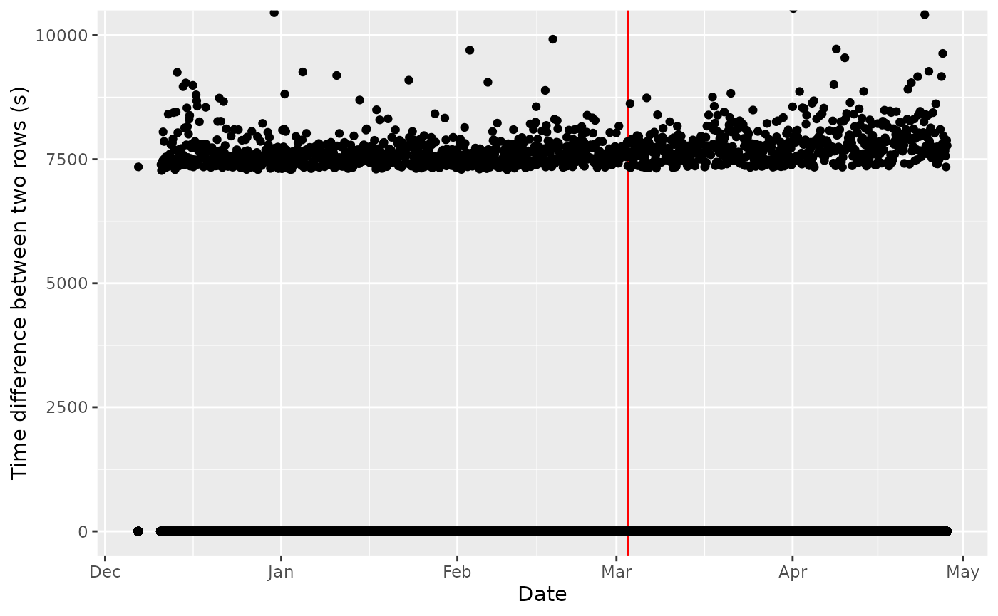

Time Gap Identification, if there were no time gap, all the dot should be at 1 second. The red line is the date when a new ’*.wch’ file has been created

Crap… We have 1459 gaps that exceed 1 s (in average of ~7959.553804s or ~2.2h). How do we deal with it? Is it the same for the other individuals?

# zoom over two days
data_plot[datetime %between% c(as.POSIXct("2015-03-01 16:07:00"), as.POSIXct("2015-03-03 16:07:00")),] %>%
  ggplot(aes(x = datetime, y = diff_time)) +
  geom_vline(xintercept = as.POSIXct("2015-03-02 16:07:00"), col = "red") +
  geom_point() +
  coord_cartesian(ylim = c(0, 10000)) +
  labs(x = "Date", y = "Time difference between two rows (s)")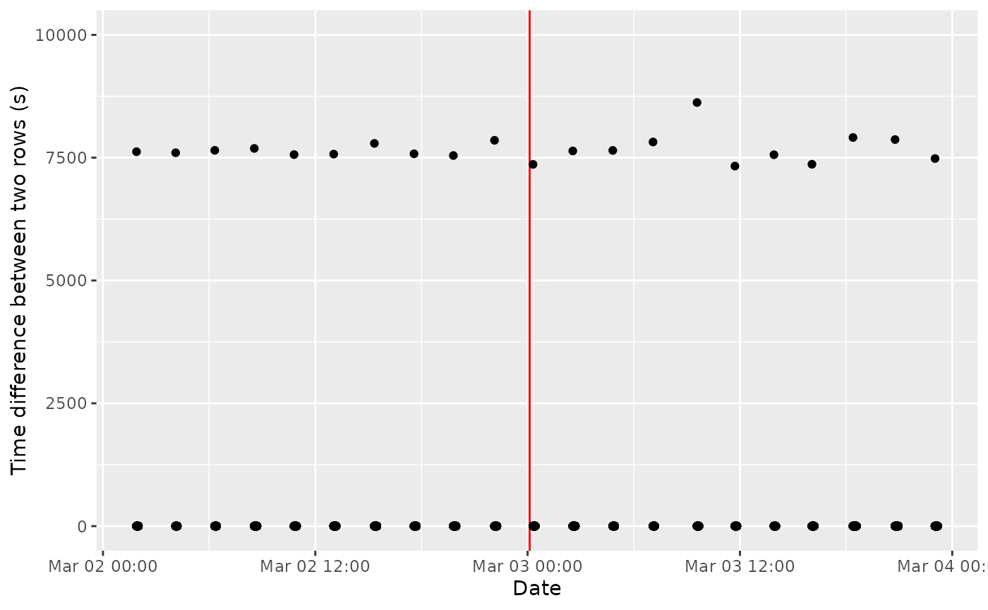

Same graph, with a zoom over two days

Well, there is clearly a pattern, I suspect the tag was programmed to be turned off every 2.2 hours?

Confirmed in Cox et al., 2017, the tag was programmed to record one complete dive every 2 hours!

# zoom over two days
ind_140075[!is.na(V2), datetime := as.POSIXct(V1, format = "%m/%d/%Y %T", tz = "GMT")] %>%
  .[datetime %between% c(as.POSIXct("2015-03-02 12:00:00", tz = "GMT"), as.POSIXct("2015-03-02 18:00:00", tz = "GMT")),] %>%
  ggplot(aes(x = datetime, y = -V6)) +
  geom_point() +
  labs(x = "Date", y = "Depth (m)")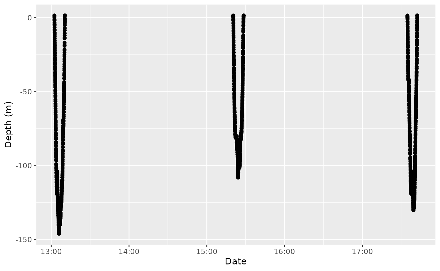

TDR over 6 hours of data recorded