Treat location data with a continuous-time state-space model

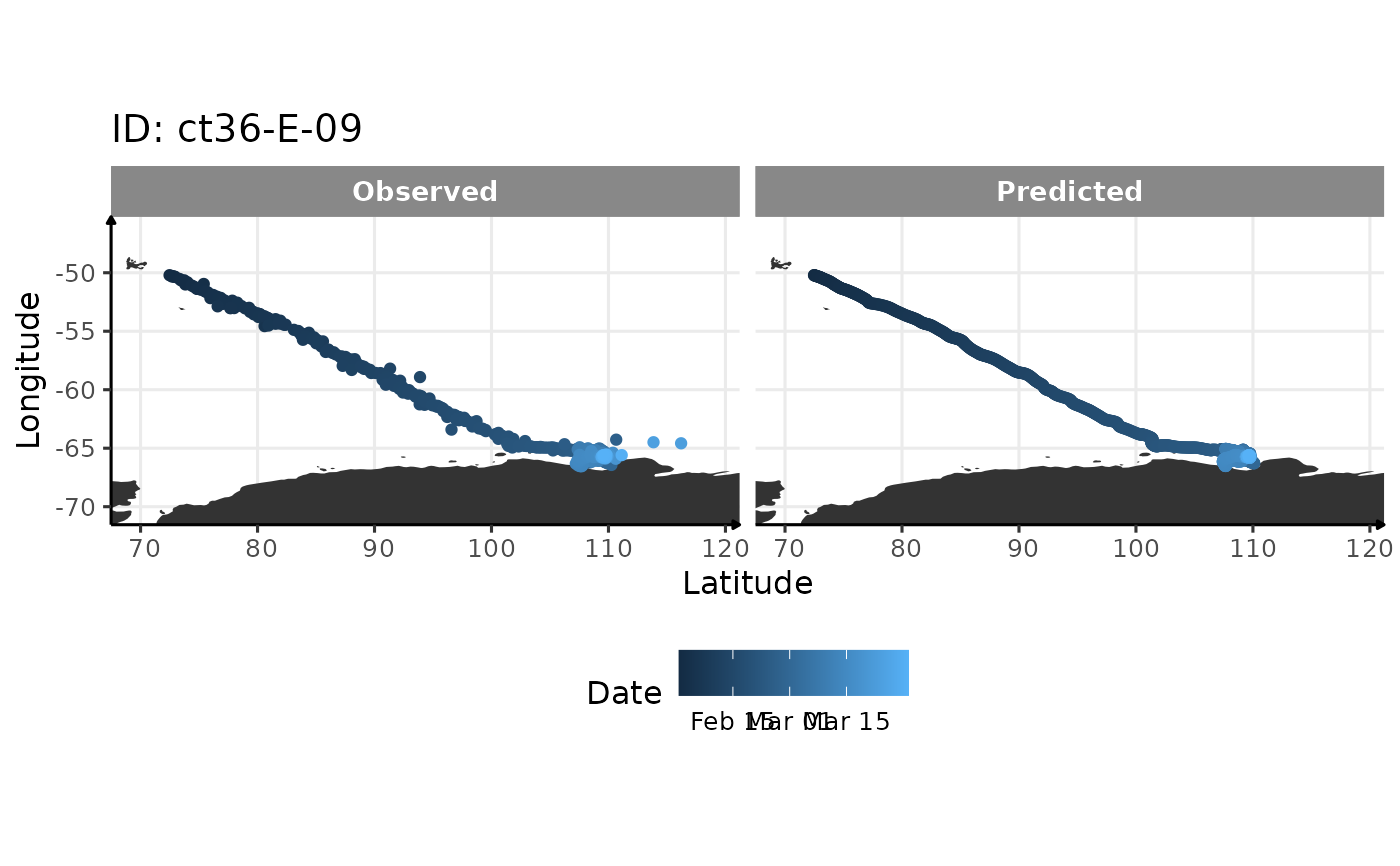
Using fit_ssm function from foieGras package, this function "clean" the location data to be used for further analysis at the dive scale.

Usage

location_treatment(
  data,
  model = "crw",
  time.step = 1,
  vmax = 3,
  with_plot = FALSE,
  export = NULL
)

Arguments

data: Dataset of observation, usually the file \*Argos.csv or \*Location.csv files
model: Choose to fit either a simple random walk (rw) or correlated random walk (crw) as a continuous-time process model
time.step: options: 1) the regular time interval, in hours, to predict to; 2) a vector of prediction times, possibly not regular, must be specified as a data.frame with id and POSIXt dates; 3) NA - turns off prediction and locations are only estimated at observation times.
vmax: The max travel rate (m/s) passed to sda to identify outlier locations
with_plot: A diagnostic plot
export: To export the new generated dataset

Value

A dataset with the new location data

References

run_foieGras_generic.R (tkeates@ucsc.edu)

https://ianjonsen.github.io/foieGras/

Examples

# load library
library(foieGras)
library(data.table)

# run this function on sese1 dataset included in foieGras package
output <- location_treatment(copy(sese1), with_plot = TRUE)
#> fitting crw...
#> 
 pars:   0 0 0 0      
 pars:   -0.07009 -0.67701 -0.73263 -0.00241      
 pars:   0.80735 -0.49698 -1.10459 0.24116      
 pars:   0.79068 -0.93408 -0.86323 0.26125      
 pars:   1.17074 -0.84805 -0.95396 0.56112      
 pars:   0.94797 -0.82123 -0.95447 0.38458      
 pars:   0.71902 -0.86148 -1.03497 0.40682      
 pars:   0.90772 -0.86547 -0.99023 0.38642      
 pars:   0.86034 -0.81931 -0.96958 0.37881      
 pars:   0.84471 -0.83656 -0.93133 0.40567      
 pars:   0.86034 -0.81931 -0.96958 0.37881